Solve By Elementary Row Operations

Return to Roadmap 2

We will solve Example 12 from the Chapter 2 Roadmap page by using elementary row operation. Start with the initial system of four linear equations in four variables.

-5x₁ + 7x₂ + 9x₃ - 11x₄	=	56	(1)
1x₁ + 2x₂ - 6x₃ - 3x₄	=	115	(2)
12x₁ - 4x₂ + 3x₃ + 8x₄	=	- 74	(3)
5x₁ - 7x₂ - 1x₃ + 4x₄	=	- 73	(4)

Once we make sure that we have accounted for all of the variables in all of the equations and that the variables are in the same order in all equations, we can represent that system of linear equations via the matrix

As noted in an earlier page and repeated here, there are a few important aspects of having the system of linear equations. First, there was no special order to the equations. We could have rearranged the order but in doing so we would end up rearranging the order of the rows in the matrix. Second, we could have multiplied any of the equations by a non-zero constant. That would change the form of the equation but not the set of points that satisfy the equation. Of course, in the matrix this would correspond to multiplying the affected row of the matrix by that same constant. And third, we could multiply, off to the side, any equation in the system by a non-zero constant and then add the resulting equation to either of the other equations in the system. In the matrix this amounts to multiplying, off to the side, a row of the matrix and then adding that result to a different row of the matrix. Those three actions are captured by three elementary row operations, rowSwap, *row, and *row+. These are built-in functions of the TI-83/84 family of calculators. The nane, syntax, and semantics of the three is given in the following table.

name	Syntax	Semantics
rowSwap(	*rowSwap(matrix name, row1, row2)*	Interchange row1 with row2 in the identified matrix.
*row(	*rowSwap(value, matrix name, row1)*	Multiply each number in row1 of the identified matrix by the given value..
rowSwap(	row+(value, matrix name, row1, row2*)	Off to the side, multiply each value of row1 of the designated matrix by the given value. Then add the resulting numbers to the numbers in row2 of the matrix. Row1 is not changed.

We will use those commands to do the elementary row operations on our calculator.

The calculator used to make the images on this page was a TI-84 Plus C. It has more resolution on the screen than do the older models in the TI-83/84 calculator. In addition, the calculator used here uses the MATHPRINT, rather than the CLASSIC option. The result is a matrix that looks more like a matrix. If you are using an older calculator, or using one in the CLASSIC mode, you will have to make some adjustment for the change in the display. However, the computations will be identical.

The process here is to change, in a step by step fashion, the given matrix to one that has 1's down the diagonal and 0's below and above those 1's. If you skip down to Figure 19 you will see that goal expressed as

This matrix, in turn, really represent four linear equations, namely,

1x₁ + 0x₂ + 0x₃ + 0x₄	=	6	(5)
0x₁ + 1x₂ + 0x₃ + 0x₄	=	11	(6)
0x₁ + 0x₂ + 1x₃ + 0x₄	=	- 10	(7)
0x₁ + 0x₂ + 0x₃ + 1x₄	=	- 9	(8)

But that is the solution, x₁ = 6, x₂ = 11, x₃ = ^–10, and x₄ = ^–9 which can be expressed as the point (6,11,^–10,^–9).

We just need to see the steps to go from the matrix

to the matrix

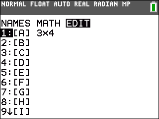
Figure 1	To get the matrix into the calculator we use the key sequence. This opens the window shown in Figure 1, and, in that window, we have moved the highlight to the EDIT position. Press to edit matrix [A].
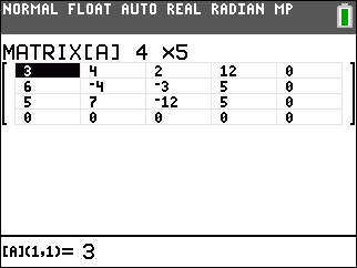Figure 2	For Figure 2 we have changed the dimensions of the matrix to hold our 4x5 matrix. The numbers shown in the matrix in Figure 2 are either 0 or values left over from an earlier matrix.
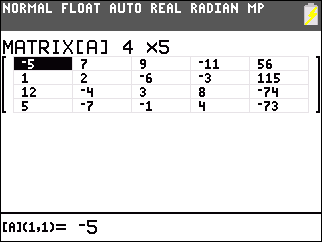Figure 3	Here, in Figure 3, we have entered all of the values from our matrix. We can leave this via the key sequence. Then we can start on the process to alter the matrix to the desired form.
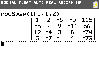Figure 4	We want to get a 1 in the first row, first column. It turns out, in the matrix in Figure 3, that we have a 1 in the second row, first column. If we swap the first and second row we will achieve our goal. We create the command rowSwap([A],1,2) to do this. Figure 4 shows the result. Remember that the matrix shown in Figure 4 is stored in the Ans, not in [A].
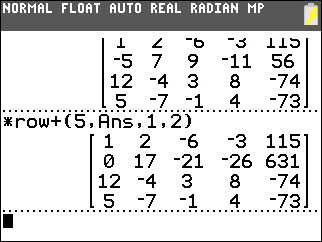Figure 5	Then we construct row+(5,Ans,1,2), using to generate Ans*, to add 5 times the first row to the second row. This produces 0 in the second row, first column. The first row remains unchanged.
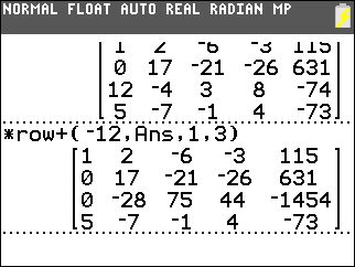Figure 6	Then we construct *row+(^–12,Ans,1,3) to add ^–12 times the first row to the third row. This produces 0 in the third row, first column.
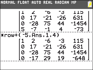Figure 7	Then we construct row+(^–5,Ans,1,4) to add ^–12 times the first row to the fourth row. This produces 0 in the fourth row, first column. Our next task is to generate a 1 in the second row, second column. We could play around, as we have in the earlier example, to find multiples of the second row and the third or fourth row that would generate that value. However, a quicker way will be to multiply the second row by 1/17*.
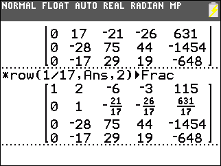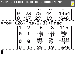Figure 8	We use *row(1/17,Ans,2) to multiply the second row by 1/17. This produces 1 in the second row, second column. Note that we appended the to the command so that the display would show fractional values rather than decimal values.
Figure 9	Then we construct *row+(28,Ans,2,3) to add 28 times the second row to the third row. This produces 0 in the third row, second column.
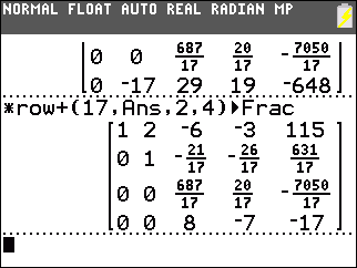Figure 10	Then we construct *row+(17,Ans,2,4) to add 17 times the second row to the fourth row. This produces 0 in the fourth row, second column. At this point we need to use the elementary row operations to produce a 1 in the third row, third column. The fastest way to do this is to multiply that third row by 17/687.
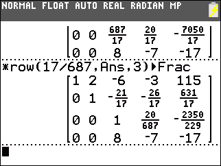Figure 11	We use *row(17/687,Ans,3) to multiply the third row by 17/687. This produces 1 in the third row, third column.
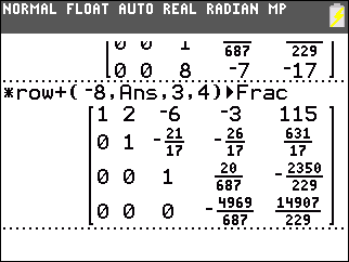Figure 12	Then we construct *row+(^–8,Ans,3,4) to add ^–8 times the third row to the fourth row. This produces 0 in the fourth row, third column.
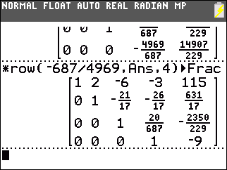Figure 13	We use *row(^–687/4969,Ans,4) to multiply the fourth row by ^–687/4969. This produces 1 in the fourth row, fourth column.
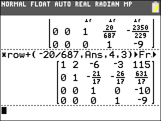Figure 14	Then we construct *row+(^–20/687,Ans,4,3) to add ^–20/687 times the fourth row to the third row. This produces 0 in the third row, fourth column.
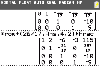Figure 15	Then we construct *row+(26/17,Ans,4,2) to add 26/17 times the fourth row to the second row. This produces 0 in the second row, fourth column.
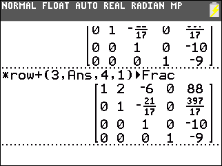Figure 16	Then we construct *row+(3,Ans,4,1) to add 3 times the fourth row to the first row. This produces 0 in the first row, fourth column.
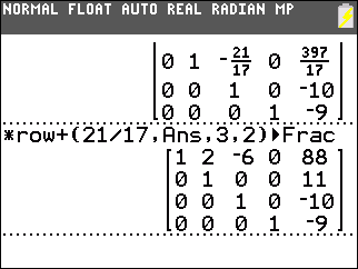Figure 17	Then we construct *row+(21/17,Ans,3,2) to add 21/17 times the third row to the second row. This produces 0 in the second row, third column.
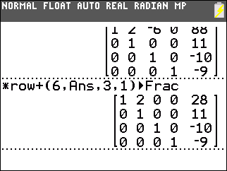Figure 18	Then we construct *row+(6,Ans,3,1) to add 6 times the third row to the first row. This produces 0 in the first row, third column.
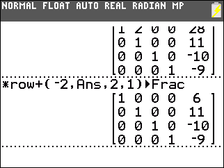Figure 19	Then we construct row+(^–2,Ans,2,1) to add ^–2 times the second row to the first row. This produces 0 in the first row, second column. We have reached our goal form. We can read the answers from this. x₁ = 6, x₂ = 11, x₃ = ^–10, and x₄ = ^–9*.