
| 3x + 4y + 2z | = | 12 | (1) |
| 6x – 4y – 3z | = | 5 | (2) |
| 5x + 7y – 12z | = | 5 | (3) |

| name | Syntax | Non-TI Symbols | Semantics |
| rowSwap( | rowSwap(matrix name, row1, row2) | Rrow1 ↔ Rrow2 | Interchange row1 with row2 in the identified matrix. |
| *row( | *row(value, matrix name, row1) | valueRrow1 → Rrow1 | Multiply each number in row1 of the identified matrix by the given value.. |
| *row+( | *row+(value, matrix name, row1, row2) | valueRrow1 +Rrow2 → Rrow2 | Off to the side, multiply each value of row1 of the designated matrix by the given value. Then add the resulting numbers to the numbers in row2 of the matrix. Row1 is not changed. |

| 1x + 0y + 0z | = | 2 | (4) |
| 0x +1y + 0z | = | 1 | (5) |
| 0x + 0y + 1z | = | 1 | (6) |


|
To get the matrix into the calculator we use the
  key sequence.
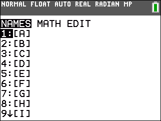
This opens the window shown in Figure 1. key sequence.
This opens the window shown in Figure 1.
|
 |
We will put the matrix into one of the ten defined matrices.
For this example we will use the [A] matrix. We use the
  keys
to move the highight to the
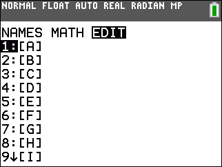
EDIT option, as is shown in Figure 2. keys
to move the highight to the
EDIT option, as is shown in Figure 2.
Because the [A] matrix is already selected we can
just press the |
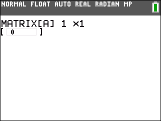 |
On this calculator we did not have a prviously defined value in [A]. Therefore, Figure 3 shows [A] as a matrix with 1 row and 1 column. |
 |
Pressing  
  changes the calculator
matrix editor from the image shown
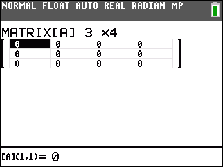
in Figure 3 to the one shown in Figure 4.
Now we need to fill in the values from our original equations. changes the calculator
matrix editor from the image shown
in Figure 3 to the one shown in Figure 4.
Now we need to fill in the values from our original equations.
|
 |
Figure 5 shows all of the values in the appropriate spots of the matrix.
We can leave Figure 5 and return the the home screen via the key sequence
  . . Now we are ready to start the pocess described above. First we want to use the elementary row operations to create a 1 in the first row, first column spot. There are many ways to do this. One way is to note that the first item in rows 2 and 3 are different by 1. If we swap the first and second row, then we will have a 6 in the first row, first column position. Then, we can add – 1 times the third row to the first row to make row 1, column 1 hold the value 1.
Our plan starts with swaping the first and second row. to do this we need to
find the rowSwap( command.
Press the |
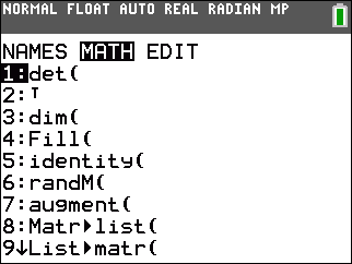 |
Figure 6 shows the list of the matrix MATH funtions. Our desired function,
rowSwap( is not to be found in Figure 6. However, if we move down the listing,
using the  key many times, we will get to
the functions shown in Figure 7. key many times, we will get to
the functions shown in Figure 7.
|
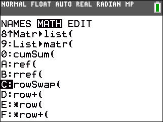 |
In Figure 7 we see the rowSwap( option, and we have highlighted it.
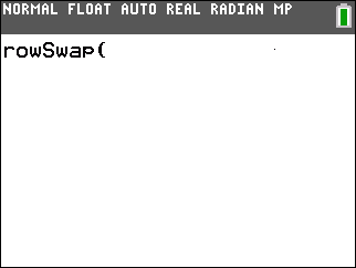
Then press the  key to paste that option
onto the main screen, as is shown in Figure 8. key to paste that option
onto the main screen, as is shown in Figure 8.
|
 |
Recall that the syntax for this command is
rowSwap(value, matrix name, row1).
We want to swap rows 1 and 2 in matrix [A]. Therefore, the desired command is
rowSwap([A],1,2). We construct that command, getting the matrix name from the
matrix menu, and then press the  key.
The reuslt is shown in Figure 9. key.
The reuslt is shown in Figure 9.
|
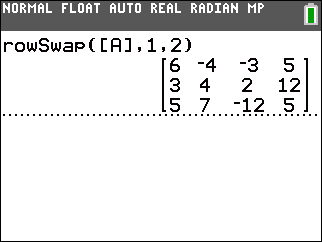 |
It is important to note that the command has been performed. It worked just as we expected, the first and second rows of the matrix have been swapped. However, the resulting matrix, the one shown in Figure 9, is stored in Ans not in [A}. In fact, the contents of [A] are unchanged. |
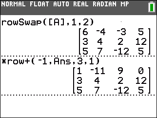 |
The next step is to multiply, on the side, row 3 of the matrix by
–1 and then add that result to row 1.
The command to do this is
*row+(‐1,Ans,3,1). form this command we
would have to return to the matrix functions list and elect the
*row+( option, then use the keys
   to continue the command. Follow that by
   to generate the Ans, then use
  
  to complete the command.
Once constructed, press
  to run the command.
All of this appears at the bottom of Figure 10. to run the command.
All of this appears at the bottom of Figure 10.
|
 |
The next number of images continue the steps of the process.
In each case, we return to the matrix function list to select
the command we want and then we complete the command following the
prescribed syntax. In all of these steps we continue to work on the matrix stored in Ans
and each command produces a new result that is then stored in Ans.
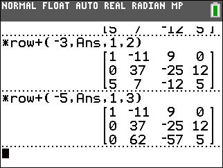
The top command in Figure 11 multiplies, on the side, the top row by –3 and adds it to the second row, thus creating a 0 in row 2, column 1. The next command multiplies, on the side, the top row by –5 and adds it to the third row, thus creating a 0 in row 3, column 1. At the end of Figure 11 we have finished the first column. Our next challenge is to get a 1 in row 2, column 2. That cell currently contains 37. |
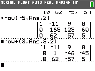 |
It may seem a little obtuse, and it is, but I happen to know that 5*37 is 185
and that 3*62 is 186. Those values differ by 1. So, we multiply row 2
by –5, using the *row( function, and then
multiply, on the side, row 3 by 3 and then add that result to row 2.
The result appears in the lower portion of Figure 12.
We have the desired 1 in row 2, column 2.
This obtuse approach is handy in that it did not require using fractions. We could have manufactured the 1 from the original 37 by multiplying row 2 by 1/37. However tht would hae introduced fractions and I prefer to avoid them for now. |
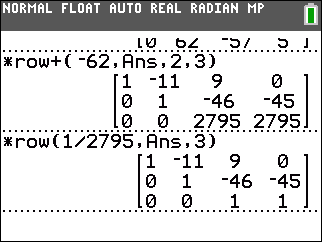 |
At the top of Figure 13 we multiply row 2 by –62
and add the result to row 3, generating a 0 in row 3 column 2.
In the lower portion of Figure 13 we multiply row 3 by 1/2795 generating
a 1 in row 3, column 3.
|
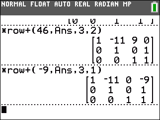 |
Multipy row 3 by 46 and add it to row 2. Multiply row 3 by –9 and add it to row 1. |
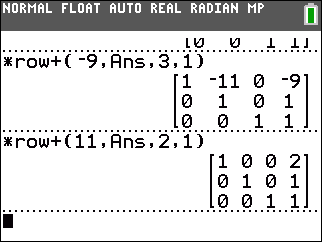 |
The upper portion of Figure 15 is just the lower portion of Figure 14. The new command in Figure 15 is to multiply row 2 by 11 and add it to row 1. The fianl result is the matrix at the end of Figure 15. As noted above, changing this back to three equations gives us x=2, y=1, and z=1. |