Introduction to Detailed Notes
This is a set of notes that have been made on reading the textbook. There
is no real attempt to have comments on absolutely everything in the
book noted here. At the same time, there is supplementary material here that
is not in the book.
After writing out the notes for the first few sections, it has become clear that there is a tendency to make this a "teaching" document. As much as possible, efforts will be made to not do this. Rather, if there is teaching material to be presented then that will be done in separate pages, with pointers inserted here.
Note that we actually did introduce irrational numbers back in Chapter 1. This is not a completely new topic. However, in this chapter we will be working with some of the irrational numbers.
On page 384, the symbol ![]()
![]() is introduced as the radical sign and the term radicand
is identified as the expression under the radical sign.
is introduced as the radical sign and the term radicand
is identified as the expression under the radical sign.
On page 386, information box #7 contains the following statement:


 if
if 
 .
.
Page 387 at the top, second line, the reference to "Section 5.5" should be to "Section 7.5".
The final sentence in the information box number 8, that starts at the bottom of page 386 and ends at the top of page 387, is
| Therefore, in this chapter all variables raised to an odd power (including 1) in a radicand are assumed to be positive when the index is even. |
Page 391. Example 3 on page 391 is extremely important. Most often we are working with square roots and we are rationalizing the denominator when that denominator is a square root. When we do this we get into the habit of multiplying both the numerator and the denominator by the sqaure root that is already in the denominator. For example, look at the steps used for reducing the the expression


|
= |
| = |
| = |
| = |
| = |
| = |
| = |
|


The book describes the classic approach to reducing roots of integers. Namely, we factor the integer into its prime factors and we use that prime factorization to pull out as many factors as possible. Converting an integer into its prime factors is a fairly mechanical process. Therefore, we should be able to write a program for our calculators to do this. (The TI-89 and 92 do this by a built-in function.) See the Prime Factors on the TI-83 for the TI-83 program and a demonstration of its use, or the Prime Factors on the TI-85/86 for the TI-85 and TI-86 programs and a demonstration of their use.
We introduce the various GETPRIME programs to aid us in reducing radicals by identifying the prime factorization of integers. We really could take this process a bit further. If we are taking the square root of a quantity, and if the prime factorization indicates that a factor of that quantity is raised to the 7th, then we know that we can reduce the radical by moving the factor to the 3rd out of the radical, leaving the factor to the 1st within the radical. For example,
 
| |
  
| |
 
| |
 
|
|
| |
| |

| |

|
There is little that the TI-83, TI-85, and TI-86 can do to help you perform the operations on radicals presented in this section. About the best that we can do is to use the calculator to check our work. We do this by having the calculator evaluate the original problem and evaluate our computed answer. The two answers should be the same. It is important to realize that this method of checking our work will ensure that our answer and the oriinal problem are equivalent. That is, we have used legal steps to change the form of the problem into a more simple form. However, we may not have changed to problem into its most simple form.
Note that there is a small difference in formulating
the expressions on the TI-83 versus the TI-85 or TI-86.
Much of this difference arises from the TI-83 automatically supplying
a left parenthesis with the radical sign.Thus, the TI-83 produces the
![]() whereas the TI-85 and TI-86
produce the
whereas the TI-85 and TI-86
produce the ![]() . In order to illustrate the
use of these commands on the various
calculators, there are numerous examples below. Each example is taken from the
text and each gives the problem, the answer, and calculator images showing the
formulation of the problem and the answer in order to evaluate both of them.
Thus, problem Q1d on page 397 is
. In order to illustrate the
use of these commands on the various
calculators, there are numerous examples below. Each example is taken from the
text and each gives the problem, the answer, and calculator images showing the
formulation of the problem and the answer in order to evaluate both of them.
Thus, problem Q1d on page 397 is


| We could evaluate these two expressions on the TI-83 as | We could evaluate these two expressions on the TI-86 as |
 |
 |
Problem Q2a is given as


| We could evaluate these two expressions on the TI-83 as | We could evaluate these two expressions on the TI-86 as |
 |
 |
Problem Q5c on page 399 is given as


| We could evaluate these two expressions on the TI-83 as | We could evaluate these two expressions on the TI-86 as |
 |
 |
Problem Q8b on page 400 is given as
| We could evaluate these two expressions on the TI-83 as | We could evaluate these two expressions on the TI-86 as |
 |
 |
Problem Q13c on page 403 is given as
|
 |
|
|
|
 |
| We could evaluate these two expressions on the TI-83 as | We could evaluate these two expressions on the TI-86 as |
 |
 |
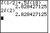
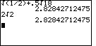
Problem Q15a on page 403 is given as
|
|
 |
 |
|
|
| We could evaluate these two expressions on the TI-83 as | We could evaluate these two expressions on the TI-86 as |
 |
 |
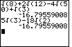
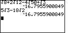
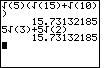
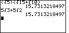
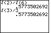
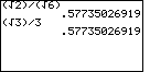
And, to demonstrate doing this work with the "cube root", we look at problem Q13d on page 403. That problem is given as
|
|
|
| We could evaluate these two expressions on the TI-83 as | We could evaluate these two expressions on the TI-86 as |
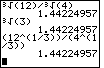 |
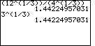 |
| Note that the image shown above computes the two expressions using the TI-83 "cube root" symbol from the MATH menu, and then the screen demonstrates computing the first expression by using the "raise it to the one third power" method. | The image above shows one way of computing the cube root on the TI-86. The TI-85 and TI-86 also have an option on the MATH/MISC submenu to do various roots. That method is not demonstrated here. |
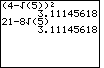
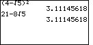
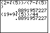
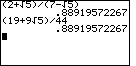
The examples given above demonstrate a method for checking our work on the calculator. owever, in each of these examples we have only been working with numbers. None of the problems demonstrated so far has involved the use of one or more variables. For example, on page 402 problem Q12b asks us to simplfy
 |
|
|
| We could assign values to X and Y, and evalue the first expression on the TI-83 as | We could assign values to x and y, and evaluate the first expression on the TI-86 as |
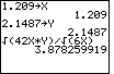 |
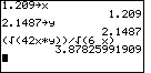 |
| Then we can evaluate the second expression as | Then we can evaluate the second expression as |
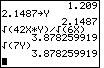 |
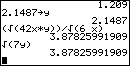 |
| Note that the image shown above uses the uppercase variables X and Y because these are the variables available on the TI-83. | The image above uses the lower-case variables x and y in part because the lower-case x is available on a single button on the TI-85 and TI-86. We couls have used the upper-case letters. It is important to be consistent within any one problem however because the TI-85 and TI-86 are case-sensitive. |
Much of this section is a repeat of the earlier work with whole number exponents. In Section 3 we extend that work to cover integer exponents. And, in Section 4 we will find that the same rules apply to rational exponents. Although we could repeat the rules here, they are stated plainly in the text.
Starting on page 416 this section of the text introduces "Scientific Notation". This has always been a useful topic for students who are going to take a physical or biological science class. Again, the text presents this material in a reasonable manner, with many examples. However, the text does not cover the use of the calculator with scientific notation or in moving between scientific and regular notation. The pages Scientific Notation on the TI-83 and Scientific Notation on the TI-85 or TI-86 give such illustrations.
Again, this section expands the rules for exponents to exponents that are rational numbers, that is, fractions. There is little that these notes can add to the material in the text. We have already introduced the idea that we can express the "nth root of a value x" on the calculator as
The text does a good job of presenting the imaginary number i, and complex numbers in the form a+bi, along with the operations of addition, subtraction, multiplication, and division with complex numbers. These are skills that are nice to have.
Note on page 436, in information box 6, the sixth line reads


 equal
equal
In many ways the calculator solves most of the problems that we need to do with complex
numbers. All of the TI graphing calculators work with complex numbers.
THe TI-83, TI-89, and TI-92 all have the imaginary number i on
the keyboard. The TI-83 uses the key sequence 
 to generate i, while the TI-89 uses the key sequence
 to generate i. The page Complex Numbers on the TI-83 demonstrates various mathematical operations
on complex numbers on that calculator.
On the other hand, the TI-85 and TI-86
take a differnt approach to complex numbers. Whereas our textbook uses the form a+bi
to show a complex number, the TI-85, the TI-86, and many textbooks use the form (a,b) to
represent the same value. That is, in one system we write 4+5i, while
in the other system we write (4,5).
to generate i. The page Complex Numbers on the TI-83 demonstrates various mathematical operations
on complex numbers on that calculator.
On the other hand, the TI-85 and TI-86
take a differnt approach to complex numbers. Whereas our textbook uses the form a+bi
to show a complex number, the TI-85, the TI-86, and many textbooks use the form (a,b) to
represent the same value. That is, in one system we write 4+5i, while
in the other system we write (4,5).
It is unfortunate that we use the same symbols for different meanings. That is,
| (4,5) | This is the symbol that we use to represent a point on the coordinate plane where x is 4 and y is 5. |
| (4,5) | This is the symbol that we use to represent an open interval of the values between 4 and 5. |
| (4,5) | This is the symbol that we use to represent the complex number that we also write in the form 4+5i. |
As noted above, the TI-85 and TI-86 use the (a,b) representation for a complex number. The page Complex Numbers on the TI-85 and TI-86 demonstrates various mathematical operations on complex numbers on those calculators.
©Roger M. Palay
Saline, MI 48176
August, 2000
