General NOTES for Math 169
Fifth Edition
Chapter 4
Introduction to Detailed Notes
This is a set of notes that have been made on reading the textbook. There
is no real attempt to have comments on absolutely everything in the
book noted here. At the same time, there is supplementary material here that
is not in the book.
After writing out the notes for the first few sections, it has become clear that
there is a tendency to make this a "teaching" document. As much as possible,
efforts will be made to not do this. Rather, if there is teaching material
to be presented then that will be done in separate pages, with pointers inserted here.
Chapter 4: Polynomials
Before we even get into this chapter it is worth looking ahead to see the
material that will follow. In particular, we will be going over essentailly the same
material a number of times. In this chapter we start with polynomials, but we
really focus on building and tearing apart trinomials, that is expressions that
look like
Ax2 + Bx + C
In Chapter 5 we will change these expressions into equations that look like
Ax2 + Bx + C = 0
We will try to solve these. We will find out that we can solve some of
these quadratic equations using the techniques of this chapter and only using
rational numbers. There will be some quadratic equations that will be
hard to solve using the techniques presented here, or that we can not solve using
just rational numbers.
We will expand our ability to manipulate polynomials in Chapter 6, and we will
look at irrational numbers in Chapter 7. In that chapter we also learn
about a new kind of number, the complex numbers. Then, in Chapter 8, we return to
solving quadratic equations such as
Ax2 + Bx + C = 0
but this time we can solve any such equation. Within the context of the rest of
this course, the importance of
qudratic expressions and equations should be clear.
4.1 Introduction
This section presents the definition and examples of many different terms, among them:
- exponent
- power
- base
- monomial
- term
- binomial
- trinomial
- polynomial
- convert to addition (definition of subtraction)
- degree of a term
- degree of a polynomial
- descending order
- ascending order
4.2 Addition and Subtraction of Polynomials
At the bottom of page 225, in box 3, the second to last line of the material contains
the statement:
Hence, –(a + b) = –a – b
I prefer to do this by using the distributive property. That is,
| – (a + b) | = |
(– 1)(a + b) |
| | = |
(– 1)(a) + (– 1)(b) |
| | = |
– a + – b |
| | = |
– a – b |
The TI-89 and TI-92 can actually do the work of adding and subtracting polynomials.
The following screen image captures the problem from page 225 in Frame 2,
(x2 + x – 7) + (2x2 – 3x + 2)
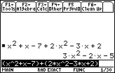 We follow that with problem Q4a from page 226 and Q5b from the bottom of that page.
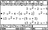 Going back to problem Q2b on page 225 requires that we use some
fairly exact problem representation. To represent 9r2t2
we will need to write
9(r^2)(t^2). The entire problem would be given as
Going back to problem Q2b on page 225 requires that we use some
fairly exact problem representation. To represent 9r2t2
we will need to write
9(r^2)(t^2). The entire problem would be given as
 The problem has been entered and performed in the following image, which has been
modified to include the red highlight.
The problem has been entered and performed in the following image, which has been
modified to include the red highlight.
 Note that we can see the left part of the problem
in the middle of the screen, highlighted by the red outline.
The entire problem is too long to be
displayed within the screen. We could move the cursor up to that line and
then scroll to the right to see the rest of the problem.
A close examination of the highlighted line reveals that
the TI-89 has already changed the problem from the way it was
entered. Note the use of exponents and the fact that
the parentheses have been removed from the problem.
The answer follows on the next line.
We can see the right part of the problem in the input area, still in the form that we
used to enter it.
Note that we can see the left part of the problem
in the middle of the screen, highlighted by the red outline.
The entire problem is too long to be
displayed within the screen. We could move the cursor up to that line and
then scroll to the right to see the rest of the problem.
A close examination of the highlighted line reveals that
the TI-89 has already changed the problem from the way it was
entered. Note the use of exponents and the fact that
the parentheses have been removed from the problem.
The answer follows on the next line.
We can see the right part of the problem in the input area, still in the form that we
used to enter it.
Unfortunately, the lower level TI calculators do not perform symbolic algebra.
Nonetheless, the TI-83, 85, and 86 can be extremely helpful in doing these
problems. In particular, we can use these calculators to check our work.
We can assign values (and we get to choose unusual values) to the variables
in the problem. Then, we can evaluate the original expression and the
answer. The two must produce the same result. For example, if we return to the
problem from Frame 2 on page 225,
(x2 + x – 7) + (2x2 – 3x + 2)
we have derived the answer as
3x2 – 2x – 5
The screen
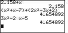 verifies that we have the correct answer for that problem.
The fact that we have the same evaluation for
both the original problem statement and for the answer DOES NOT PROVE
that we have the correct answer. However,
getting the same evaluation for the two expressions supports
our belief that we have not introduced errors by our work.
Furthermore, because we chose a strange value
for x, we can be quite confident that it it not an accident that
the two expressions produce the same value.
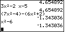
The next problem we will look at uses the variable x again.
Therefore, we can continue to use the strange value that we
had put into x earlier. The next figure demonstrates the correctness of
the answer for Q4a on page 226, where we simplified
(7x2 – 4) – (6x2 + 2)
to be x2 – 6.
verifies that we have the correct answer for that problem.
The fact that we have the same evaluation for
both the original problem statement and for the answer DOES NOT PROVE
that we have the correct answer. However,
getting the same evaluation for the two expressions supports
our belief that we have not introduced errors by our work.
Furthermore, because we chose a strange value
for x, we can be quite confident that it it not an accident that
the two expressions produce the same value.
The next problem we will look at uses the variable x again.
Therefore, we can continue to use the strange value that we
had put into x earlier. The next figure demonstrates the correctness of
the answer for Q4a on page 226, where we simplified
(7x2 – 4) – (6x2 + 2)
to be x2 – 6.
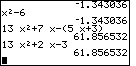
 We continue our work by looking at the solution for Q5b where we have the problem
13x2 + 7x – (5x + 3)
and our answer 13x2 + 2x – 3.
We continue our work by looking at the solution for Q5b where we have the problem
13x2 + 7x – (5x + 3)
and our answer 13x2 + 2x – 3.
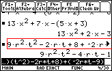
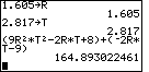
When the problem uses variables other than "x" we need to assign
strange values to the new variables. Problem Q2b on page 225
uses the variables r and t.
In that problem we needed to simplify
(9r2t2 – 2rt + 8) + (– 2rt – 9)
to produce the answer
9r2t2 –4rt – 1
A TI-86 was used to produce the image below.
To save keystrokes, we have used the variables R and T.
There was only enough room on the calculator screen to show the strange values
being assigned to the variables, and the evaluation of the original problem.
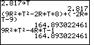
 The next screen shows the evaluation of the answer, again indicating that our
answer is correct.
The next screen shows the evaluation of the answer, again indicating that our
answer is correct.
Using the calculator to verify our work is an extremely
powerful technique. Although the TI-85, 86, and 83 do not do the problem
for us, they make checking our work a straight-forward task. It is a task that
should be done on every such problem.
4.3 Multiplication of Polynomials
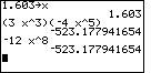
Again, one of the benefits of the TI-89 and TI-92 is that those
calculators can do symbolic algebra. For example, problem Q1a
on page 227 is
(3x3)(– 4x5)
with the answer being – 12x8
On the TI-89 we can do this as shown in the following image.
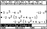 However, on that same image above, we also tried problem Q5d from page 229, namely,
– 2y2(3y2 + 4y – 1)
which should have given an answer of
– 6y4 – 8y3 + 2y2
It is clear from the image above that the calculator did not do the work that
we expected. In fact, the TI-89 needs to be told to expand the problem to
give a solution.
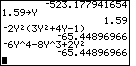
In the input section, the next image contains almost all of the command to do this.
we need to give the command
expand((– 2y^2)(3y^2+4y-1))
which is just one character too long to be shown in its entirety in the input area.
However, on that same image above, we also tried problem Q5d from page 229, namely,
– 2y2(3y2 + 4y – 1)
which should have given an answer of
– 6y4 – 8y3 + 2y2
It is clear from the image above that the calculator did not do the work that
we expected. In fact, the TI-89 needs to be told to expand the problem to
give a solution.
In the input section, the next image contains almost all of the command to do this.
we need to give the command
expand((– 2y^2)(3y^2+4y-1))
which is just one character too long to be shown in its entirety in the input area.
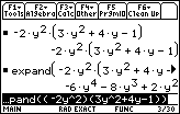
 The command that was started above is concluded below, and it has been
entered into the calculator. Note that the command appears in the history area,
and that it is now followed by the answer.
The command that was started above is concluded below, and it has been
entered into the calculator. Note that the command appears in the history area,
and that it is now followed by the answer.
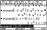
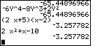
As a final example of the power of the expand function on the TI-89,
the following image shows the work for Q10e on page 231, namely, showing that
(2x + 5)(x – 2) expands to be
2x2 + x – 10
Where the TI-89 performs symbolic multiplication, the TI-83, 85, and 86
can be used, as before, to check our work.
[There is a program for the TI-85 and 86 that will perform the
multiplication of two polynomials, assuming that we have polynomials of one variable.
However, learning to use that program is probably much more complex than is
learning the procss of multiplying polynomials by hand, except for
the case of long polynomials.]
Again, we place some strange value
into the variables being used in the problem, and then we can enter
both the problem statement and the
solution that we are checking. The two expressions need to produce the same values.
We will look at screens that check the same problems shown above.
We return to the problem
(3x3)(– 4x5)
with the answer being – 12x8
The next image demonstrates producing a value for both the problem and the answer.
We use the next screen to check
– 2y2(3y2 + 4y – 1)
and its answer
– 6y4 – 8y3 + 2y2
Finally, to verify the problem
(2x + 5)(x – 2) as compared to its answer
2x2 + x – 10
we look at the next screen.
It is important to remember that this section is dealing with the
process of multiplying any two polynomials. Thus, we can use the
techniques presented in this section to multiply
(4x3 + 7x2 – 5x + 9)(– 8x2
+ 3x – 11)
However, most of the time we are asked to multiply much more simple polynomials.
In particular, we are often asked to multiply polynomials that we might
expresss as (Ax + B)(Cx + D)
Let us just do this one problem,
using A, B, C, and D in place of numbers. If we distribute the left factor over the right
we get Ax(Cx + D) + B(Cx + D)
Ax(Cx) + Ax(D) + B(Cx) + B(D)
A(C)x2 + A(D)x + B(C)x + B(D)
A(C)x2 + (A(D) + B(C))x + B(D)
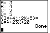
Now, if we take a problem that has numeric coefficients, such as
(3x + 4)(2x + 5)
then we have A=3, B=4, C=2, and D=5. Thus,
the answer will be
3(2)x2 + (3(5) + 4(2))x + 4(5)
6x2 + (15 + 8))x + 20)
6x2 + 23x + 20
This process is so straight-forward that it almost begs us to write a program for
the calculator to do this work. We will have to give the calculator four numbers representing
A, B, C, and D, and it will compute and display
three numbers representing F, G, and H in
Fx2 + Gx + H
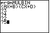
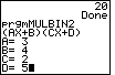
The listing of a TI-83 program, called MULBIN, to do this is given below.
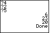
 And a sample run of the program is given in the following two frames:
The MULBIN program presented above does exactly the
computations that we determined in our earlier work.
A user of the program must know exactly what to enter and the exact
meaning of the output.
And a sample run of the program is given in the following two frames:
The MULBIN program presented above does exactly the
computations that we determined in our earlier work.
A user of the program must know exactly what to enter and the exact
meaning of the output.
The program MULBIN2 is an enhancement of the MULBIN program. This new version
merely makes the output a bit easier to read. After getting the values
from the user, the MULBIN2 program first constructs and displays the original problem
and then it constructs and displays the answer. The following two frames
demonstrate the MULBIN2 program.
The MULBIN and
MULBIN2 programs are available for the TI-83.
In addition, there are versions for the TI-85 called
MULBIN.85P and
MULBIN2.85P, and versions for the TI-86 called
MULBIN.86P and
MULBIN2.86P.
There are no versions for the TI-89 because that calculator
already handles these problems directly, as was illustrated above.
4.4 Special Products
There are few things worth memorizing in most of mathematics. However, these
special products happen so often that they are worth the effort. First,
the square of a binomial:
(a + b)2 = a2 + 2ab + b2
Some times students will try to memorize that formula and the following one
(a – b)2 = a2 + 2ab + b2
However, I prefer to change (a – b)2 into
(a + – b), and then recognize that we have
the same formula that we had before. Therefore,
(a – b)2
becomes
(a + – b)2
which expands to
a2 + 2a(– b) + (– b)2
which we then simplify to
a2 + – 2ab + b2
The product of the sum and the difference of two values will be used
over and over again. The formula states
(a + b)(a – b) = a2 – b2
We need to recognize that the formula gives us the "rule" and that we
can apply that rule whenever we have the product of the sum and the
difference of two values. Thus,
(3x4y + 5xy2)(3x4y – 5xy2)
becomes (3x4y)2 – (5xy2)2
which simplifies to
9x8y2 – 25x2y4
The book goes on to give two more special products.
These will be useful later, but mostly when we are using them backwards.
For now, there is nothing to do but to memorize them, knowing that they will be on
just about every test that covers this material. In fact, they are used on such tests
precisely because they are so weird that "knowing the answer" is a good indication
that a student has studied the related material. The two special products are
(a + b)(a2 – ab + b2) = a3 + b3
and
(a – b)(a2 + ab + b2) = a3 – b3
Again, each formula represents a "rule" or a "pattern" that we can follow.
Thus, the problem
(2x3 – 3y2)(4x6 + 6x3y2 + 9y4)
becomes
(2x3 – 3y2)((2x3)2 + (3x3)(2y2) + (3y2)2)
which, by the formula above, becomes
(2x3)3 – (3y2)3
which simplifies to
8x9 – 27y6
4.5 Factoring Polynomials
The method for factoring a trinomial (over integers) that is presented on pages 245 through
254 is called "splitting the middle term". In order for us to do that method,
we need to first multiply the coefficient of the x2 term by the
constant term. Then we look at the factors of that product, and
we select the factors that have the appropriate sum or difference that
equals the coefficent of the middle term.
Thus, for the problem
15x2 – 14x – 8
we multiply 15 times – 8 to get – 120.
In order for the constant term to be negative, we
must be multiplying a positive by a negative. Thus, we want to find two factors
of 120 that have a difference equal to – 14.
Unfortunately, it is a bit of a pain to find all of the factors of 120.
It would be nice if we had a way to do this.
We could create a program on the calculator that produces
a list of the possible pairs of factors for any given number.
such a program has been created and it is
described on the FACTPAIR
web page. Having the list of factors for a given number
simplifies the task of "splitting the middle term".
Of course, if we can get the calculator to find factor pairs, then
we should be able to get it to find the factor pair with the
desired sum or difference. We could give such a program the values of
A, B, and C in
Ax2 + Bx + C
and the program could
- compute A*C as the number to use to find the factor pairs
- look at the sign of C to determine if we want the sum or difference
- look at B as the desired sum or difference
- find the factor pair of A*C that gives the desired sum or difference
- Assuming that a factor pair is found, split the middle term
- take the common factor from the left pair and the right pair of terms
- complete the factoring to produce (Lx+M)(Px+Q)D
- display those values
This is the algorithm, the set of steps, that we use when we perform the
"split the middle term" process. Each step can be done on the calculator.
The web page TRINOMIAL FACTORIZATION lists, describes,
and gives examples of using the trifact1 program that
implements the algorithm outlined above.
The major problem with the trifact1 program is that the output is ugly.
We need to interpret the five numbers as L, M, P, Q, and D in
(Lx+M)(Px+Q)D
The TI-83, 85, and 86 do not make it easy to get pretty looking outut, but it
can be done. The web page
TRINOMIAL FACTORIZATION, version 2
lists, describes, and gives examples of using such an enhanced program,
called trifact2.
The change from trifact1 to trifact2 is merely the change required to
make the output look nice. The algorithm to "split the middle term" does
not change.
At this point in the course, the most frequent question asked is "Can
I use the programs for the test?" The answer is "Yes". I would like you to
be able to do the problems by hand, at least the easier ones. However,
if you have a tool (the calculator with the program) to do the work, and
you know how to use that tool, then by all means, use it.
4.6 Perfect Squares and Completing the Square
The first few pages of this section
are really a replay of the "Special Products" and the "Factoring Polynomials" sections.
That is, we already knew that we had the two "rules" for the special products:
(a + b)2 = a2 + 2ab + b2
(a – b)2 = a2 – 2ab + b2
Now we are reading these backwards. If we find a polynomial that
fits the form on the right, then we can factor that polynomial to be
the product on the left.
The work starting on page 264 leads us into the process called "completing the square".
This is a complex task that requires a certain amount of algebraic manipulation
to transform a problem from one that we can not factor using our earlier methods, to
one that we can factor. The process itself is important to understand, mostly because
we want to apply it once to a general problem so that we can get a general answer.
In order to prepare us for that step the book presents the "completing the square"
methodology and then asks us to practice it on specific problems.
4.7 Sums or Difference of Two Squares and Two Cubes
Again, this section is really using the rest of the "Special Products" rules
(a + b )(a – b) = a2 – b2
(a + b)(a2 – ab + b2 = a3 + b3
(a – b)(a2 + ab + b2 = a3 – b3
but using them backwards, taking problems that conform to the forms on the right and
using the equivalence to factor those forms to the products on the left.
In this work we see that x2 + y2 is not factorable.
However, in some special cases we can factor things that look somewhat like
x2 + y2.
©Roger M. Palay
Saline, MI 48176
June, 1999