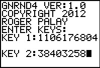
We need to start with some data.
We will generate a list of data on the calculator using
GNRND4 with Key 1=1106176804 and Key 2=38403258. That list
will be the same numbers that appear in the following table:
Thus, our problem will be to generate a histogram for the data in the
list above.
Figure 1
|
We begin by running the GNRND4 program with the given key values.
|
Figure 2
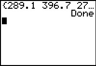 |
This produces the list of values that we want.
We recall that those values are stored in
L1.
|
Figure 3
 |
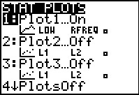
Use   to open the STAT PLOTS
menu. Here we see that Plot1 is set to display a histogram using the data
in L1. This is just what we want. to open the STAT PLOTS
menu. Here we see that Plot1 is set to display a histogram using the data
in L1. This is just what we want.
Press  to move to the ZOOM menu. to move to the ZOOM menu.
|
Figure 4
 |
Now we move down the menu to find the desired ZoomStat option.
Once it is highlighted, press  to perform that option. to perform that option.
|
Figure 5
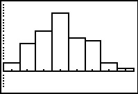 |
The calculator examines the data in L1
and then it creates a histogram based on those values.
We can inspect the valeus that the calculator used by moving to the
WINDOW screen (press  ). ).
|
Figure 6
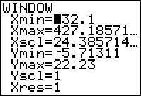 |
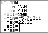
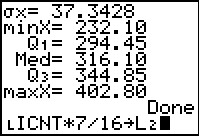
Here ae the values being used. In particular, the
lower limit of the first class of values is 232.1 (the leading 2 is covered by the blinking cursor).
the width of each class is 24.385714... and, if there were an additional class beyond the 8
needed to cover the values in L1 then that additional class
would start at 427.18571... That value is the effective upper limit of the last class in
our histogram.
We can decide to change these values if we want a slightly different structure
for our histogram.
|
Figure 7
 |
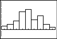
We have set these values so that the start of the historgram is at 230,
the width of each class is 20, and the effective upper limit of the final class is
410.
|
Figure 8
 |
Having set new WINDOW values in Figure 7, we press
 to get the new histogram shown in Figure 8.
Both the histogram of Figure 5 and the histogram of Figure 8 are correct. The difference
is the choice of lower limits and the class width. The only advantage related
to the histogram of Figure 8 is that the lower limit and width are nice, even values.
As demonstrated in earlier pages, we could actually shift into "trace" mode and find the number
of items in each of the classes (columns) shown in Figure 8. However, we will take the slightly easier
approach of using the COLLATE3 program to do this for us. to get the new histogram shown in Figure 8.
Both the histogram of Figure 5 and the histogram of Figure 8 are correct. The difference
is the choice of lower limits and the class width. The only advantage related
to the histogram of Figure 8 is that the lower limit and width are nice, even values.
As demonstrated in earlier pages, we could actually shift into "trace" mode and find the number
of items in each of the classes (columns) shown in Figure 8. However, we will take the slightly easier
approach of using the COLLATE3 program to do this for us.
We have conveniently skipped over the real problem here. We have had the calcualtor
produce a histogram but we have not talked about our producing one. We will return to this
issue in Figure 33.
|
Figure 9
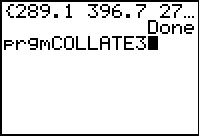 |
We exit the graph mode and select the COLLATE3
program from the list of programs.
|
Figure 10
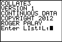 |
When we run the program it asks us for the
location of the data. We give it L1.
|
Figure 11
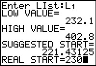 |
The program gives us the low and high values in our data and asks for the starting point
of the histogram.
As we did with the earlier histogram we will set that starting point to
be 230.
|
Figure 12
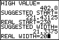 |
The progream gives a suggested width, but we had already made up our
mind to use the value 20. We respond with that value.
|
Figure 13
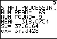 |
Figure 13 shows some of the display output from the program.
|
Figure 14
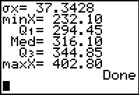 |
Figure 14 shows the rest of the display output from the program.
|
Figure 15
 |
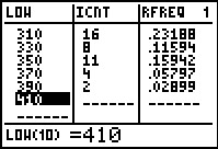
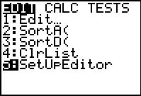
We have seen the COLLATE3 program before. We know that it creates
other lists while it does its work. We move to the STAT
menu and then open the Stat Editor to see those values.
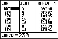
This gives, for each class, the LOW values,
the count of values in the class (i.e., the frequency), and the
relative frequency of those counts.
|
Figure 16
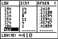 |
We can run down the list to see the remaining
class values. Note that the LOW list has an extra element
holding the lower limit of the next class if it were there.
|
Figure 17
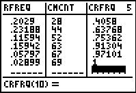 |
Moving the cursor to the right allows us to see two of the remaining
lists in the display. CMCNT holds the cumulative
count of values, while CRFRQ
holds the cumulative relative frequencies.
|
Figure 18
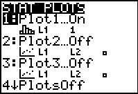 |
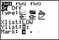
As you may have noted in our earlier work, the histogrm is not the only style of graph that the calculator
can do. We will create a relative frequency graph from the output lists of
COLLATE3. Since those lists are already in the calculator, we return to the
STATS PLOT menu via .
We want to change Plot1 and that the choice that is highlighted so
we just press .
|
Figure 19
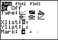 |
Figure 19 shows the Plot1 screen after we changed it to
select the line chart (second chart option on the top line of charts) and
we have moved the cursor to follow the Xlist: field. The
current value of that is L1.
We want to use the LOW values as the Xlist:. To do this we can either type the characters of
the name or move to the LIST menu
and select the LOW entry there. This latter option is shown in Figure 19a.
|
Figure 19a
 |
Selecting LOW from the list of lists.
|
Figure 20
 |
We want the Ylist:
to be RFREQ so that we have a graph that shows the
relative frequency. Again, we can type the name, note
that the calculator os already in "alpha" mode, or we can return to the
LIST menu
and select the desired name.
|
Figure 21
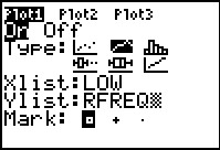 |
Figure 21 shows the screen with all the changes made.
Press to move to the ZOOM menu.
|
Figure 22
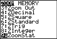 |
On the ZOOM menu, move down to highlight the ZoomStat option.
Press to perform that option.
|
Figure 23
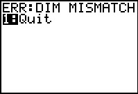 |
The result is an error! We read the error message, ERR:DIM MISMATCH
and press to choose the Quit option, there being no other choice.
So what went wrong? We have actually seen the cause of the error, and even commented on
it, although we did not recognize it as a problem at the time. We have asked the calculator to create a graph
based upon pairs of values in two lists,
LLOW and LRFREQ.
The problem is that the program COLLATE3 put an extra value into
LLOW. We noted this in Figure 16. When I wrote
COLLATE3 I thought that it would be helpful to add that extra value
so that it would be easy to find the upper limit
of the last class. However, that means that the two lists,
LLOW and
LRFREQ have different numbers of elements.
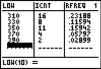
This is the DIM MISMATCH of the error message. We no longer need the extra value
in LOW. Therefore, the easiest fix to this problem is to remove that value.
|
Figure 24
 |
We return tot he Stat Editor, move down to the extra value in LOW,
and then press  to move to Figure 25. to move to Figure 25.
|
Figure 25
 |
Having fixed the problem, we return to the ZoomStat option,
shown in Figure 26.
|
Figure 26
 |
Press to have the calculator perform the action.
The result is a relative frequency chart as chown in Figure 27.
|
Figure 27
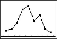 |
This is the relative frequency chart that we wanted.
If, on the other hand, we want a chart of the
cumulative relative frequency, an Ogive chart, then all we need to do is
set Plot1 to use the list CRFRQ.
|
Figure 28
 |
To do this we return to the STAT PLOTS menu and select Plot1.
|
Figure 29
 |
On the Plot1 screen we change the Ylist: value to be CRFRQ.
|
Figure 30
 |
We will need to have the calcualtor redo its
analysis and reset the appropriate
WINDOW values. To accomplish this we return
to the ZOOM menu and again select and perform ZoomStat.
|
Figure 31
 |
Here we have a cumulative frequency chart for our data, remembering that we really
have the cumulative relative frequency of the classes into which we divided all of the original
data.
|
Figure 32
 |
If we press  to enter trace mode, and then move
to the right three times, we have highlighted a point on the chart.
That point corresponds to the value 290 with a cumulative relative frequency of 0.4057971.
We should recall that we chose the Xlist: to be the values in LOW
and that is what the calculator is reporting. However, we are really looking at
0.4057971 as the relative frequency of original data
points through the fourth class, the class that runs from 290
to just before 310. to enter trace mode, and then move
to the right three times, we have highlighted a point on the chart.
That point corresponds to the value 290 with a cumulative relative frequency of 0.4057971.
We should recall that we chose the Xlist: to be the values in LOW
and that is what the calculator is reporting. However, we are really looking at
0.4057971 as the relative frequency of original data
points through the fourth class, the class that runs from 290
to just before 310.
|
Figure 33
 |
As indicated above in the discussion tied to Figure 8, although we have
produced a histogram on the calculator, we do not know, at this point, how high to make each bar
if we are actually drawing a histogram. We did look at this problem
in a much earlier page dealing with bar charts.
The same logio applies here.
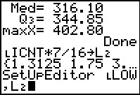
If we pick any particular column, say the column representing
the class from 310 to just before 330, and we decide to have that column in
the histogram be 7 centimeters tall, then all other columns
must be in proper proportion given their
respective frequencies. The class from 310 to almost 330 has 16 values in it.
Therefore, for any other class we can find its required height
by taking its frequency times 7 and dividing by 16. We can do this all at once
with the command
LICNT*7/16
We have constructed such a command at the bottom of Figure 33 and then assigned the result to
be stored in
L2. (We get the name of the list from the LIST
menu and then complete the command with the appropriate keys.)
|
Figure 34
 |
After performing the command that we created in Figure 33 we return to the
STAT menu to get to the SetUpEditor command, which we then select.
|
Figure 35
 |
In this case we want to create the command
SetUpEditor LLOW,L2
We return to the LIST menu to get the LLOW name.
|
Figure 36
 |
We find the LOW name and press .
|
Figure 37
 |
Then we complete the command via

 . Finally, press
to perform the command. . Finally, press
to perform the command.
Then when we re-open the Stat Editor
it will show those two lists.
|
Figure 38
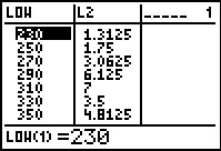 |
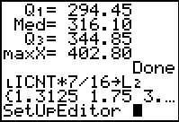
Here we see the start of the two lists. From this we can tell that
the height of the claas from 230 to just before 250 needs to be 1.3125 centimeters.
The height of the claas from 250 to just before 2570 needs to be 1.75 centimeters.
All of this based upon our first establishing that we wanted the height of the class from
310 to just before 330 to be 7 centimeters, and that is the value shown here.
|
Figure 39
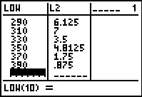 |
Finally, we move down to see the required height of each of the remaining classes.
|