Steps to a Linear Regression on the TI-89

This page is not a complete introduction to finding linear regressions on the TI-89. Rather, this is a quick tour of the processes needed to generate the graphs that are in the text at the start of Chapter 2, Section 3. Additional material related to regression in general can be found on the Linear Regression page. Additional work on doing regression on the TI-89 can be found on the Linear Regression on the TI-89 page.

In the text we are given the following table

x (miles)	3	5	9	11	12	15	20	25
y (time)	6	9	13	16	16	21	28	31

and we are asked if the data is related. Then the text gives a plot of the data points and eventually draws the line of best fit for those data points. On this page we will develop those same plots with the same points and the same line.

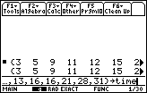
Figure 1	Figure 1 captures the data input near the end of the process. The values for the "miles" list have already been entered, although the input and the response lines are truncated on the right. Then, the values for the "time" list are entered in the command and data input line, and the list is assigned to "time". In this case, the left side of the statement is no longer visible on the screen. We will need to press the key to accept the command and move to Figure 2.
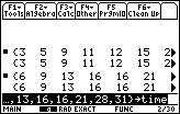
Figure 2	The result of pressing ENTER is shown in Figure 2. We could use the cursor keys to move the highlight up to one of the history lines and then use the right cursor key to examine the complete line. However, for this page we will accept that the data has been entered correctly.
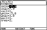
Figure 3	We will do a little preparation work before we process and display the data from our two lists. In particular, we would like to be able to plot the values in the list. We will need to set the "WINDOW" values in the graphing calculator to handle the values in our lists. Press to open the WINDOW screen, shown in Figure 3. Figure 3 displays the current limits to the WINDOW values. These are the values that were last used on this particular calculator. If we look back at our two lists, we see that none of the pairs of values will fall into our current setting. Therefore, we will want to change those settings.
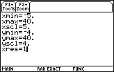
Figure 4	Changing the xMin to ^–5, the xMax to 40, and the xScl to 5 will handle the MILES list, and having yMin set to ^–4, yMax set to 40, and yScl set to 4 will handle the TIME list values.
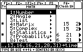
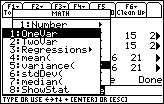
Figure 5	We could press to accept the value for xres, press to return to the HOME screen, and then press to open the MATH menu shown in Figure 5. Of the options shown here we want to select item #6, Statistics. To do this we press the key.
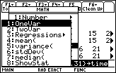
Figure 6	Selecting Statistics just opens a new window, shown in Figure 6. The item that we want here is the "Regressions" option. Thus, press to move to the next Figure.
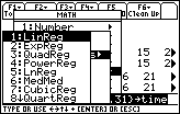
Figure 7	Yet another window has been presented. This one has the command that we want to use, namely, LinReg. We can press to select that command.
Figure 8	As a result, all of the pop-up windows have been closed and the command LinReg has been pasted into the data and command input line. However, the command is not complete. We need to tell the calculator the names of the lists to use in the computation of the linear regression.
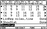
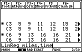
Figure 9	In Figure 9 we have completed the command as: LinReg miles,time We can press to move to Figure 10.
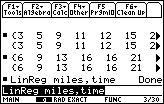
Figure 10	Figure 10 tells us that the calculator has completed the computation. Unfortunately, the calculator does not seem to be willing to show us the answers. It merely states that the work is "Done".
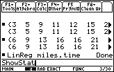
Figure 11	To see the answers, we need to give another command, namely, ShowStat. We press to re-open the MATH menu. Ans we press to open the Statistics window, as shown in Figure 11. Here we can see that ShowStat is item number #8 in the list. Therefore, we press to select that command and move to Figure 12.
Figure 12	We tell the calculator to perform the command by pressing the key. The result appears in Figure 13.
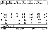
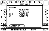
Figure 13	The small pop-up window in Figure 13 contains the even smaller results of the previous Statistics computation, namely, LinReg miles,time. We should compare these results with those produced by a TI-86 and given in the text, There are a number of important differences here. First, the parameters "a" and "b" have reversed meanings on the two calculators. On the TI-86 "a" is used as the intercept value, and "b" is used as the slope. In the TI-89, using the LinReg command, the "a" is used for the slope and the "b" is used as the intercept value. Second, the TI-86 has a few extra digits of accuracy. This is not a major problem. THe six decimal digits given by the TI-89 are more than enough for any of our purposes. And, third, the TI-89 output gives the "R²=" value while the TI-86 gives "n=", the number of items in each original list. Again, these are not major issues. We can always go back to find the number of items in the lists, and the "R²=" value is merely the value of the "corr" squared.
Figure 14	Now that we have the regression equation parameters, let us go back and create the plot of the data points. Then we will draw the regression equation on the same graph. We return to the HOME screen by pressing the key.
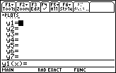
Figure 15	Then, we move to the Y= screen shown in Figure 15 by pressing the keys.
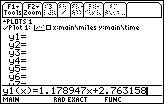
Figure 16	At this point we do not want to define an equation. Rather we want to specify a plot. Therefore, we will use the key to move the highlight up to select Plot1. One there, we press the key to select that particular Plot. The result is the new window shown in Figure 17.
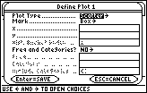
Figure 17	In the new window, the options are already set for a "Scatter" plot and for the use of a "Box" to mark each data point. However, we need to specify the two lists to use for the "x" and "y" values.
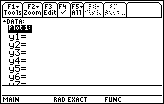
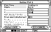
Figure 18	In Figure 18 we have used the key to move down the items and we have entered "miles" as the list of "x" values, and we have entered "time" as the list of "y" values. We can press to accept that last value, and then to "SAVE" the values that we have entered.
Figure 19	Having SAVEd the values in Figure 18, the calculator returns to the Y= screen. Now the Plot1 line has the values specified in the previous screen. We move to the next Figure by pressing the keys.
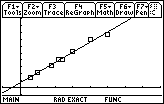
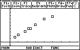
Figure 20	Figure 20 is the graph of the data points. It looks remarkably similar to the graph in the text, allowing for the difference between graphs on the TI-86 and the TI-89. Now we want to add the regression equation.
Figure 21	We use the keys to return to the Y= screen. There we can enter the regression equation using the values that we found back in Figure 13.
Figure 22	Press to accept the regression equation specified in Figure 21, and to go back to the GRAPH screen where we can see both the data points and the graph of the regression equation.