TI-83: Simple 3 equation 3 variable
The main page for solving systems of linear equations on the TI-83 and TI-83 Plus.
The previous example page covers a Simple 2 equation 2 variable situation
but with missing and other varaibles.
The next example page covers a Simple 4 equation 4 variable situation,
with an integer solution.
WARNING: The TI-83 and TI-83 Plus are almost identical in terms of the material presented here.
The major difference is the labels that are on certain keys. The TI-83
has a  key, whereas on the TI-83 Plus
requires 2 keys to achieve the same result, namely, the
key, whereas on the TI-83 Plus
requires 2 keys to achieve the same result, namely, the

 key.
The text below will be done from the perspective of the TI-83. That is, all
reference to the MATRIX key will be demonstrated via the
key. If the user has a TI-83 Plus then the key strokes should be
.
To save some space, and to ignore this difference, the numeric keys
(the gray ones) have been changed here to only show the key
face, as in
key.
The text below will be done from the perspective of the TI-83. That is, all
reference to the MATRIX key will be demonstrated via the
key. If the user has a TI-83 Plus then the key strokes should be
.
To save some space, and to ignore this difference, the numeric keys
(the gray ones) have been changed here to only show the key
face, as in  .
In addition, the
.
In addition, the  key will be shown as
  and the
key will be shown as
and the
key will be shown as  , again to save space.
The problem we will use on this page is
2x - 6y + z = 18
-4x + 7y + 5z = 7
3x - y + 8z = 29
We are looking for the values of the variables that make all three equations true.
[Remember that
these are linear equations in three variables. In Cartesian space, each equation
represents a plane. There are an infinite number of points on each plane, and
an infinite number of solutions to the individual equations. Two planes can
cross and their intersection is a line. Any point on that line is a solution to
for both equations. Three planes can intersect in a point.
That point of intersection is a solution to all three equations.
It is the only point that solves all three equations. We need to find that point, that
x, y, and z value that solve all three equations.]
Before we start using the calculator, note that these equations are given in standard form.
That is, they appear as Ax + By + Cy = D,
where A, B, C, and D are numeric values.
For three equations, in three unknowns (variables) x, y and z,
we could write the equations in a general
standard form as:
Ax + By Cz = D
Ex + Fy + Gz = H
Ix + Jy + Kz = L
As we will see, the calculator uses a more general standard form for these equations, namely:
a1,1 x1 + a1,2 x2 + a1,3 x3= b1
a2,1 x1 + a2,2 x2 + a2,3 x3= b2
a3,1 x1 + a3,2 x2 + a3,3 x3= b3
This new form can be more confusing in simple cases, such as two variables and two equations,
but it is more useful in complex situations, such as 7 variables and 7 equations. The
key to understanding this general form is that the numbers after the a's indicate first the
equation (row) and second the variable to which the numeric coefficient is attached. Thus,
a2,1 indicates that this is the number in the second equation attached
to the first variable. The variables are numbered by the subscript of x,
so x1 represents the first variable and
x3 represents the third variable. The constants on the right side of the
equations are numbered by the equation (row) in which they appear. Therefore,
b1 is the constant for the first equation and
b3 is the constant for the second equation.
The problem that we were given was:
2x - 6y + z = 18
-4x + 7y + 5z = 7
3x - y + 8z = 29
and we remember that the general standard form on the calculator is:
a1,1 x1 + a1,2 x2 + a1,3 x3= b1
a2,1 x1 + a2,2 x2 + a2,3 x3= b2
a3,1 x1 + a3,2 x2 + a3,3 x3= b3
so, for this problem
| a1,1 is 2 | x1 is x |
a1,2 is -6 | x2 is y |
a1,3 is 1 | x3 is z |
b1 is 18 |
| a2,1 is -4 | x1 is x |
a2,2 is 7 | x2 is y |
a2,3 is 5 | x3 is z |
b2 is 7 |
| a3,1 is 3 | x1 is x |
a3,2 is -1 | x2 is y |
a3,3 is 8 | x3 is z |
b3 is 29 |
Special note should be given to a1,3 above. In the first
equation, 2x - 6y + z = 18 the coefficient of
the variable z is understood to be 1 and is not written.
However, in the table above we
specifically remember and indicate that the coefficient is the value "1".
A similar situation appears in the third equation where the coefficient of the
variable y is understood to be -1, accounting for the implied 1
and the subtraction. Thus, in the table above, a3,2 is -1.
The calculator uses a matrix to hold a rectangular array of numbers. There are two ways to
enter a matrix into the calculator. First, you can use the [ and ] characters to type
the matrix directly into the calcualtor. That method is demonstrated in Figure 1 below.
Second, the calculator has a Matrix Editor that you can use to enter values into a matrix.
That method was demonstrated in the 2 variable, 2 equation page.
The other Figures on this page are used to demonstrate
how the calculator produces the reduced row echelon form of the given matrix.
With all of that out of the way, we are finally ready to start using the calculator.
The steps shown before assume that the calculator is turned on, that we are not in any
menu, and that the screen is clear.
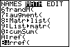
Figure 1
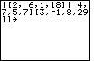
| In Figure 1 we enter the desired matrix directly from the calculator keyboard.
To do this we use the  to generate a [
to signal the start of the matrix. A second
produces a [ to signal the start of a row. Then we give the coeeficients and the constant of
the row, separated by commas. The keys for our example are to generate a [
to signal the start of the matrix. A second
produces a [ to signal the start of a row. Then we give the coeeficients and the constant of
the row, separated by commas. The keys for our example are


 .
Then we use .
Then we use  and to produce ][
to signal the end of the first row and the start of the second row, respectively. The
values in the second row are
and to produce ][
to signal the end of the first row and the start of the second row, respectively. The
values in the second row are 

 .
We use
and to produce ][
to signal the end of the second row and the start of the third row, respectively. The
values in the third row are
.
We use
and to produce ][
to signal the end of the second row and the start of the third row, respectively. The
values in the third row are
 .
Then, we need to end the third row with a ], and end the matrix with a ].
We do this with the keys
and .
Finally, we want to store this matrix on the calculator. We start to store it
by pressing the .
Then, we need to end the third row with a ], and end the matrix with a ].
We do this with the keys
and .
Finally, we want to store this matrix on the calculator. We start to store it
by pressing the  key. key.
|
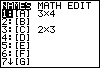
Figure 2
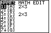
| On a TI-83 or a TI-83 Plus we need to store a matrix into one of the 10 predefined matrices,
[A], [B], [C], [D], [E], [F], [G], [H], [I], or [J]. To do this we need to find
the name of the desired matrix. The names are available in the MATRIX menu. On the TI-83 we press the
key to open the MATRIX menu. (As noted at the start of this page,
on the TI-83 Plus we use the sequence
keys to accomplish the same thing.)
Figure 2 shows the MATRIX menu. The calculator used here already has a matrix stored in [A]
and another matrix stored in [C],
in fact, both matrices have 2 rows and 3 columns. We will store our matrix in place of the
matrix already in [A].
To do this, we can press the key to select the [A] matrix name.
|
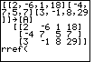
Figure 3
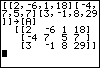
| Figure 3 shows the result of our work in Figure 2. The name [A] has been appended to the store command
in our screen. We created the
command that defines the matrix and assigns it to [A]. To perform that command we press the
key.
Performing the command stores the matrix into [A] and
then displays it on the screen as  This is the form that the TI-83 uses to display a matrix.
|
Figure 4
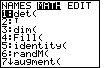
| Our next step is to find the reduced row echelon form of this matrix.
We could do this ourselves, using what are known as
elementary row operations. However, the TI-83
has a function that will try to produce the reduced row echelon form of the original matrix.
That command is rref(). We can find this command in the MATRIX menu. Therefore,
we open that menu again, via the key, and then move to the MATH
submenu via the
 key. Unfortunately, the rref( option does not appear
on this screen. We will need to use the key. Unfortunately, the rref( option does not appear
on this screen. We will need to use the  key to move the selector highlight
down the list of options until we find the desired option, shown in Figure 4a. key to move the selector highlight
down the list of options until we find the desired option, shown in Figure 4a.
|
Figure 4a
| In Figure 4a we have located the rref( function. Press to select that option
and paste rref( onto the main screen.
|
Figure 5
| The full command that we want to construct is rref([A]).
In Figure 5 we have the start of this command. Now we need to append the name of our matrix.
To do this we will need to open the MATRIX menu again. Press
to move to Figure 6.
|
Figure 6
| Once again, the list of matrix names is presented.
Note that the dimensions for [A] have changed.
[A] is already highlighted.
Therefore, we can press
to select [A] and move to Figure 7.
|
Figure 7
| Once [A] has been pasted into the command,
we press  to complete the
comamnd, as shown in Figure 7.
All that remains is to press
to get the calculator to
perform the function and to produce
the reduced row echelon form of the
original matrix [A]. to complete the
comamnd, as shown in Figure 7.
All that remains is to press
to get the calculator to
perform the function and to produce
the reduced row echelon form of the
original matrix [A].
|
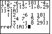
Figure 8
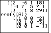
| Finally, we have the reduced row echolon form of the original matrix.
This new form appears as
 remember that this is merely a shorthand version of the three linear equations
1x + 0y + 0z = – 2
remember that this is merely a shorthand version of the three linear equations
1x + 0y + 0z = – 2
0x + 1y + 0z = – 3
0x + 0y + 1z = 4
and those equations tell us that x=– 2, y=– 3,
and z=4.
That point, the point (– 2,– 3,4),
is the solution to the original problem.
|
The main page for solving systems of linear equations on the TI-83 and TI-83 Plus.
The previous example page covers a Simple 2 equation 2 variable situation
but with missing and other varaibles.
The next example page covers a Simple 4 equation 4 variable situation,
with an integer solution.
©Roger M. Palay
Saline, MI 48176
May, 2001