Figure 1
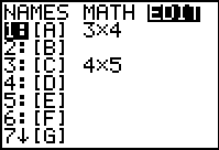
| Open the matrix menu and move to the editor. We will use [A]
for this problem.
|
Figure 2
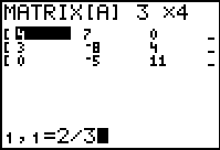
| [A] already has the correct dimensions for the current problem, namely 3 rows and 4 columns.
In Figure 2 we have moved to enter a new value into row 1, column 1 of the matrix.
The new values, 2/3 is the coefficient of the first variable, x, in the first equation.
In Figure 2 we have entered the value but have not yet hit the ENTER key to really submit the new value.
Press the  key to move to Figure 3. key to move to Figure 3.
|
Figure 3
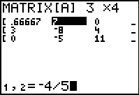
| In Figure 3 we can see that the first coefficient has been entered into the matrix.
We might note that the display of that value has just a few digits. This is for display only. Were we to return
to that first row, first column spot we
would see, at the bottom of the screen, the full precision of the value. A similar situation
is discussed below in Figure 4. Meanwhile,
Figure 3 has us entering the next coefficient, –4/5 at the bottom of the screen.
Press the  key to move to accept that value and move forward with the problem. key to move to accept that value and move forward with the problem.
|
Figure 4
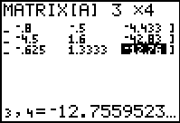
| To get here we have entered all of the coefficients and constants from
the original problem, for all three equations.
The last value that we entered was –2143/168.
It went into row 3, column 4, the currently highlighted cell in the matrix.
Note that the matrix display of this is now –12.76, but this is just a short version of the value.
The longer version is given at the bottom of the screen as –12.7559523... but even that has more digits
on the calculator than are displayed three. [You could press  to move the cursor to the
number at the bottom of the screen and then use the to move the cursor to the
number at the bottom of the screen and then use the  key to move over to display more
digits if need be.] key to move over to display more
digits if need be.]
|
Figure 5
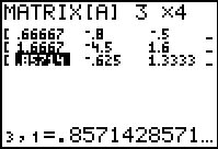
| For Figure 5 we have merely used the  key to move the display so that we can verify the values
in the first column, which was not shown in Figure 4. Note that all the values in the display are in decimal format.
At this point, having entered all the values from the problem into the matrix,
we can quit the matrix editor by pressing key to move the display so that we can verify the values
in the first column, which was not shown in Figure 4. Note that all the values in the display are in decimal format.
At this point, having entered all the values from the problem into the matrix,
we can quit the matrix editor by pressing   . .
|
Figure 6
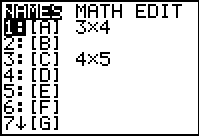
| Once out of the matrix editor, we return to the matrix menu so that we can select the
name of the matrix for display. To leave this screen, since [A] is the current selection,
press the  key. key.
|
Figure 7
| The action of Figure 6 just pasted the nameof the matrix onto our main
screen. We would like to see the matrix, but in fractional form. Therefore, press the
 key to open the MATH menu as shown in Figure 8. key to open the MATH menu as shown in Figure 8.
|
Figure 8
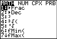
| We want the first item in the menu,  . Therefore, just press the . Therefore, just press the
 key to paste that command onto the main screen, as shown in Figure 9. key to paste that command onto the main screen, as shown in Figure 9.
|
Figure 9
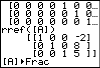
| Here our command is set up. Press  to tell the calculator to perform the
command. to tell the calculator to perform the
command.
|
Figure 10
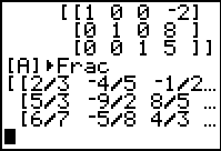
| The calculator has displayed the matrix, or at least the left side of the matrix, using fractional
notation for the entries. As usual, we can use this display to verify the entry of the
values of the current problem.
|
Figure 11
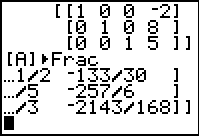
| We can move to the right side of the matrix using the
 key. key.
|
Figure 12
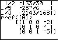
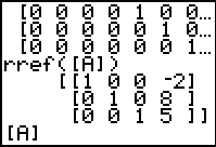
| We can recall the command rref([A]) and then use the
 key to perform the command, resulting in
Figure 12. From this we could reconstruct the transformed equations as
1x + 0y + 0z = –2 key to perform the command, resulting in
Figure 12. From this we could reconstruct the transformed equations as
1x + 0y + 0z = –2
0x + 1y + 0z = 7
0x + 0y + 1z = –5
or x=–2, y=7, and z=–5
or we could give the solution as a point (–2,7,–5).
|


 key to move to Figure 3.

 key to move to accept that value and move forward with the problem.

 to move the cursor to the
number at the bottom of the screen and then use the
  key to move over to display more
digits if need be.]

 key to move the display so that we can verify the values
in the first column, which was not shown in Figure 4. Note that all the values in the display are in decimal format.
At this point, having entered all the values from the problem into the matrix,
we can quit the matrix editor by pressing
 .
.

 key.
key.

 key to open the MATH menu as shown in Figure 8.

 key to paste that command onto the main screen, as shown in Figure 9.

 to tell the calculator to perform the
command.


 key.
key.

 key to perform the command, resulting in
Figure 12. From this we could reconstruct the transformed equations as
 key, whereas on the TI-83 Plus
requires 2 keys to achieve the same result, namely, the

 key.
The text below will be done from the perspective of the TI-83. That is, all
reference to the MATRIX key will be demonstrated via the
 .
In addition, the
  key may be shown as