TI-83: Complex 3 equations in 2 variables, non-intersecting

The main page for solving systems of linear equations on the TI-83 and TI-83 Plus.
The previous example page covers a Simple 4 equation 4 variable situation, with no unique solution.
The next example page covers a Complex 3 equations in 2 variables, 2 parallel, no unique solution.

WARNING: The TI-83 and TI-83 Plus are almost identical in terms of the material presented here. The major difference is the labels that are on certain keys. The TI-83 has a

key, whereas on the TI-83 Plus requires 2 keys to achieve the same result, namely, the

key. The text below will be done from the perspective of the TI-83. That is, all reference to the MATRIX key will be demonstrated via the

key. If the user has a TI-83 Plus then the key strokes should be

. To save some space, and to ignore this difference, the numeric keys (the gray ones) have been changed in some places to show the key face, as in

. In addition, the

key may be shown as

and the

key may be shown as

, again to save space.

The problem we will use on this page is -2x + y = 0
4x - 9y = -14
1x + 3y = 28 Having looked at the previous examples of using the "rref" function on the calculator, we should recognize that this problem is different from all of the earlier problems. In those problems we always had exactly the same number of equations as we had variables. For example, in the previous page we had 4 equations in 4 variables. Here we have just two variables, but we have 3 equations.

One could use the "rref" function with any size matrix, but it is intended to be used, as we have seen, for situations where we have the same number of equations as we have variables. In a real sense, we have an extra equation here. If we only had two equations then we could use "rref" to find their point of intersection. Let us move ahead in that direction. At first we will restrict our analysis to the first two equations:

-2x + y = 0
4x - 9y = -14

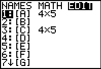
Figure 1	Open the matrix menu and move to the editor. We will use [A] for this problem.
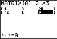
Figure 2	[A] does not have the correct dimensions for the current problem. We need to change those dimensions to be 3x2 to hold the two equations each with two coefficients and a constant. Not seen in Figure 2 is the four under the blinking cursor, although we know it is four since there are four rows in the matrix.
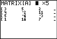
Figure 3	For Figure 3 we have changed the dimensions of the matrix and we have entered all of the values to represent our two equations.
Figure 4	Use to exit the matrix editor and return to the main screen.
Figure 5	Use to recall the previous command.
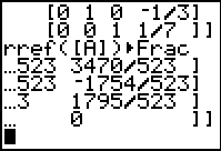
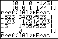
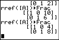
Figure 6	Press to perform the command. The response is shown in Figure 6. From this we see that for the two equations -2x + y = 0 4x - 9y = -14 have become 1x + 0y = 1 0x + 1y = 2 That is, the two lines intersect at the point (1,2). Now we will look at the third equation along with the second equation.
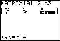
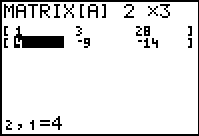
Figure 7	To do this we just need to return to the matrix editor and change a row of values. This has been done in Figure 7.
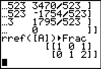
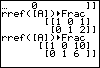
Figure 8	To solve that system of equations, we return to the main menu and recall the previous command and then perform it. The result is shown in Figure 8. the two equations 1x + 3y = 28 4x - 9y = -14 have become 1x + 0y = 10 0x + 1y = 6 That is, the two lines intersect at the point (10,6). This is a different point of intersection than we had witht he first two equations. Therefore, the three equations cannot possibly intersect in one point.
Figure 9	So far we have looked at the system of the first and second equations and the system of the third and second equations. From that inspection we know that there is not a single point where they all intesect. It is not necessary to find out where the first and third equations intersect, but it cannot hurt. We return to the matrix editor, replace the second equation values with those of the first equation. This change is shown in Figure 9.
Figure 10	Returning to the main screen, recalling the command and performing it shows that the first and third equations intersect at yet a different point, (4,8).
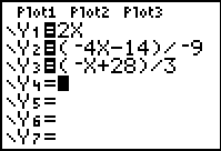
Figure 11	Especially in this case, it is instructive to go ahead and just graph the three equations. Moving to the Y= screen, we have entered the three equations into the calculator. Note that the "style" of this entry is one of convenience rather than to duplicate the slope-intercept form of the equation. The calculator does not care if the equation is in the formal y=mx+b format.
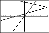
Figure 12	Recognizing that the points of intersection are (1,2), (10,6), and (4,8), we know that we will get a good graph using the Zoom Standard setting. This has been done in Figure 12. There we can see that the three lines intersect pairwise in the expected points.
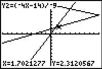
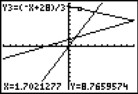
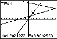
Figure 13	This figure, and the two subsequent figures merely provide the trace information for the three equations on the graph. We use the key to move from equation to equation in the graphs.
Figure 14
Figure 15