Probability: Introduction

Return to Topics page

Topics to be covered on this extremely long and dense page: Probability, or at least understanding probability, is an essential tool in understanding and using inferential statistics. That requirement causes us to stop talking about statistics for a while and instead talk about probability.

Spoiler Alert: Although understanding probability is essential to understanding inferential statistics, the breadth and depth of the topic presented here far exceeds that required for the inferential statistics that will be presented in this course. However, the course syllabus, and for the most part the syllabus for just about every college level introductory statistics course, includes all of the probability topics that will be presented here.

Probability, as a subject matter, is quite different from statistics. Being different, this material may require different learning strategies. Be aware that we are changing directions here and that you may have to self-assess your own mastery of this material in a slightly different way.

In order to talk about probability we will have to introduce a number of new terms with new definitions. For example, we want to differentiate between tasks that are deterministic and tasks that yield a result, but one where we do not know what that result will be.

Computer programs are a form of a deterministic task. The goal of a computer program is to take the information that is presented to the program and manipulated that information to produce new information. A requirement of a computer program is that no matter how many times you run the program, if you start with the same initial conditions, the same initial information, the computer program will produce the same new information. For example, we have a computer program that reads all of the registration and grade records for a student at WCC and from that information the program computes and prints the GPA for the student. No matter how many times we run the program, if we give it the same information it produces the same GPA. Of course, if a grade is chaged, or there are new grades added for noew courses for the student , then the program will produce a newly computed GPA. The result is determined by the initial information and the process defined by the computer program.

An example of a non-deterministic task is to pour out 7 M&M's from a freshly opened bag of the candy, and count the number of dark brown pieces that are in the 7 morsels. We can repeat this task any number of times, each time with the same initial condition (a fresh bag of M&M's, but there is no expectation that we will get the same result each time. [We will get 7 pieces each time, because we are careful. But the colors of the pieces will almost certainly change from one instance of the task to the next.]

Although I personally like the term non-deterministic task, the more common phrase used in statistics for this is to call such a task an experiment. It is important to note that this is a highly specialized use of the word experiment. In statistics when we say something is an experiment we mean that it is a non-deterministic task. It is something that we can repeat again and again, each time getting a result, but where we can never be sure, before we run the experiment, of the exact result that we get.

Some experiments can be quite simple. Flipping a coin and seeing if it comes up heads or tails is an experiment. Tossing a pair of dice and counting the dots showing on their tops when they come to rest is an experiment. Drawing names out of "hat" is an experiment. Each of these has an initial condition, an action or actions that can be performed to produce a final condition, and a measurement or evaluation that characterizes that final condition where the measurement or characterization is not predictable.

Some experiments can be more complex. Starting with 100 coins arranged in a row, flipping all 100 coins, keeping them in their same position in the row, and determining the longest "run" (consecutive occurrences) of "tails" is an experiment. Toss three red and two blue dice, look at the top faces and count the dots on each. First compare the highest red to the highest blue. If the red value is larger then record -1B otherwise (if red is equal to or less than blue) record -1R. Second compare the second highest red to the remaining blue. Again, if the red value is larger then record -1B otherwise (if red is equal to or less than blue) record -1R. Third, consolidate the results so a case of -1B and -1B becomes -2B and a case of -1R and -1R becomes -2R, but the case of -1B and -1R remains as is. This is an experiment. In fact it is the rule for doing battle of three attacking armies against two defending armies in Hasbro's game called Risk. We always perform the same task, roll three red and two blue, but the result is not determined until we actually roll the dice.

An experiment can be performed many times. A trial is just one of those times. If we are flipping a coin to see if we get heads or tails, then a trial is one flip. If we are drawing names from a hat, then a trial is one draw. If we are flipping 100 coins to see the longest "run" of tails then one flip of the 100 coins is a trial. If we are playing Risk and have three attacking armies in combat against two defending armies, then one roll of the three red and two blue dice is a trial.

Each trial in an experiment has an outcome. The collection of all possible outcomes is the sample space. For flipping a coin to see if it comes up heads or tails, the sample space is the set {H,T}, H for heads, T for tails. For drawing names out of a hat, the sample space is the set of all the different names that we put into the hat. For our battle in Risk, the sample space has three possible values which we represent as the set {-2R, -2B, -1R and -1B}. For flipping the 100 coins and looking for the longest run of tails the sample space has 101 possible outcomes. We could get 100 heads in which case the longest run of tails would be 0. we could get many different combinations of the 100 coins where the longest run is 1 tail. The same is true for getting 2 tails as the longest run, and so on up to the case where we could get 100 tails. We could represent this sample space by the set {0T, 1T, 2T, 3T,...,99T, 100T}. Notice that the sample space includes all possible outcomes, even those that we really would never expect to see.

We will use the term random variable to mean a variable, i.e., something that holds a value though the value may change in different instances, that has a value in the sample space for our current problem.

The sample spaces just discussed were all from performing a single trial of the experiment. We get more complicated sample spaces when we run more than one trial. For example, we could flip a coin twice. Then the possible outcomes, the sample space, become {HH, HT, TH, TT}. Although in casual speech we may say the outcomes are two heads, two tails, or a head and a tail, our sample space differentiates HT from TH. Therefore, in the case of flipping three coins the sample space is {HHH, HHT, HTH, HTT, THH, THT, TTH, TTT}.

There are times when it is helpful to actually write out a sample space, just so that we can see all of the possibilities and perhaps count how many of certain outcomes appear in the sample space. Please see the Look at a Sample Space page for an example or two.

Consider the experiment that starts with five different letters and has the process of making an arrangement of just three of them as the first three characters on a license plate. This is to be done with the understanding that once we have selected a letter it is no longer available to be used again. Remember that the order of the letters on the license plate is important. We will assume that the letters are A, B, C, D, and E. Then our sample space is {ABC, ABD, ABE, ACB, ACD, ACE, ADB, ADC, ADE, AEB, AEC, AED, BAC, BAD, BAE, BCA, BCD, BCE, BDA, BDC, BDE, BEA, BEC, BED, CAB, CAD, CAE, CBA, CBD, CBE, CDA, CDB, CDE, CEA, CEB, CED, DAB, DAC, DAE, DBA, DBC, DBE, DCA, DCB, DCE, DEA, DEB, DEC, EAB, EAC, EAD, EBA, EBC, EBD, ECA, ECB, ECD, EDA, EDB, EDC}. That s right, there are 60 different ways to arrange 5 letters taken 3 at a time. Such arrangements are called permutations. Look at the Permutations page for more details and examples.

A completely different experiment would be to use those same five letters but to allow a letter to be used more than once. Thus there would be 5 choices for the first position, five for the second, and five for the third. We would get three letter sequences from AAA through EEE. There would be 5x5x5=125 such possible values, many more than the 60 we saw above. It is worth noting that the number of possible outcomes increases dratically with an increase in the available choices and/or with an increase in the number of "positions" to fill. Thus, if we start with 8 letters, ABCDEFGH, instead of the 5 used above the number of possible outcomes goes from 125 to 8x8x8=512. Alternatively, if we stay with the 5 letters, ABCDE, but we have 4 spots to fill we get outcomes from AAAA to EEEE and there will be 5x5x5x5=625 such outcomes. Finally, if we start with 8 letters, ABCDEFGH, and we have 4 spots to fill then we will have outcomes from AAAA to HHHH and there will be 8x8x8x8=4096 such outcomes.

Now consider the experiment that starts with five different people and has the process of forming a committee of just three of them. Notice that the order of people on a committee is not important. We will assume that the people are A, B, C, D, and E. Then the sample space is {ABC, ABD, ABE, ACD, ACE, ADE, BCD, BCE, BDE, CDE}. There are 10 different 3 person committees that we can form from 5 people. You should note that BAC is not listed in the sample space. That is because BAC is the same committee as ABC, which is already in the sample space. The order of people on the committee is not important. Such formations, where order is not important, are called combinations. Look at the Combinations page for more details and examples.

Wrapping up our new terms for the moment, we define an event. In the most simple case, and event is just one of the items in the sample space. A more complicated event can be made up of multiple items in the sample space. For example, our experiment involving flipping three coins and recording the result, thus having the sample space {HHH, HHT, HTH, HTT, THH, THT, TTH, TTT}, a simple event would be to have the result be HTH. A more complex event using the same experiment would be to have the number of heads be more than the number of tails, or to find any one of HHH, HHT, HTH, or THH.

So, what have we defined so far? In all of this we have yet to discuss probability. We assign a non-negative number to each item in the sample space such that the sum of all these assigned values is 1. This number is the probability of having that item be a simple event for one trial of the experiment. In the most straight-forward case, each item in the sample space has the same probability. In that situation, if there are N items in the sample space then the number assigned to each item must be 1/N. The most simple example of this is flipping one coin. The sample space is {H,T} and, assuming this is a fair coin, the assigned probability is 1/2 or 0.5 for each outcome. We denote this with the statement P(X=H)=0.5 and P(X=T)=0.5, meaning that the probability of the event of having the outcome, X, be equal to H is 0.5, and the probability of the event of having the outcome, X, be equal to T is 0.5.

It is important to note that probability must be between 0 and 1, inclusive. If you are working on a problem and you compute the answer to be a probability that is greater than 1 or less than 0 then your answer is wrong.

It is also important to realize that the sum of all of the probabilities for the items in the sample space must be 1. This concept is used over and over in our work in statistics. It means, among other things, that if we know that the probability of an event is 0.38 then the probability of getting a result that is not in the event is 1-0.38, that is, 0.62.

Looking at a second example, if the experiment is to flip a coin three times, recording the sequence of heads or tails, then we know that the sample space is {HHH, HHT, HTH, HTT, THH, THT, TTH, TTT}. If each item in the sample space has the same probability then the probability for any one result must be 1/8=0.125. Thus, the probability of getting, on one trial, the result HTT must be 0.125, and we write this as P(X=HTT)=0.125.

Events can be more complex. Staying with the experiment of flipping a coin three times, we could look at the event of getting exactly two tails. In symbols this appears as P(X=getting exactly two tails), and that value will be the sum of the probabilities of all of the individual items in the sample space that make up the event. In this case, the items HTT, THT, and TTH are all part of the event. Therefore, P(X=getting exactly two tails)=1/8+1/8+1/8=3/8=0.375.

It is not necessary to have an equal probability for all of the items in the sample space. Rather than "flip" a coin we can "spin" a coin. Methods for doing this will be shown in class. In spinning a coin we insist that the coin spin on a flat, even surface and that it spins for at least 3 seconds. For most coins, and especially for older, worn coins, the probability of getting heads is not 1/2 (and, therefore, as we know, the probability of getting tails is not 1/2 since the two have to add to a sum of 1). However, the probability of getting heads for one coin is not necessarily the same as the probability of getting heads on another one, even if the two coins are of the same denomination or even if they are from the same year.

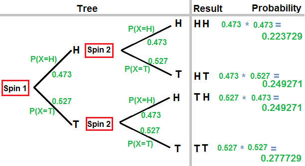
Let us say that we have a particular coin, a US penny from 2000. It turns out that for that particular coin P(X=heads)=0.473, which means that the P(X=tails)=0.527. How can we use that information to find the probabilities to assign to each of the outcomes in the sample space {HH, HT, TH, TT} associated with the experiment of spinning the coin twice? One way to do this is to look at a tree diagram. The tree diagram for spinning our specific coin twice is given in Figure 1.

Figure 1

To compute the probability for any one entry in the sample space we follow the tree to that event multiplying the probabilities that we find along the path.

Below, in Figure 2, we have a more complex tree diagram, this one with three possible outcomes. Please note that each time this page is loaded or refreshed the probabilities of the different outcomes changes. Therefore, the probabilities at the of each item in the sample space, listed to the right of the tree, also change.

Figure 2 (changes on reload)


The tree shown in, and the underlying experiment behind, Figure 2 is based on the idea of replacement. What happens if we do not replace the selected item?

Another situation, one where sampling is done without replacement is shown in Figure 3. Because the items are not replaced, successive terms in the computation of the probabilities will have decreasing denominators, and in cases where an item has been chosen before, smaller numerators. Note that in the interest of making the tree easier to follow the fractions in Figure 3 have not been reduced to lowest terms.

Figure 3 (changes on reload)


So far we have seen sample spaces and probabilities assigned to outcomes which in turn lead us to probabilities assigned to more complex events. But where do we get the simple probabilities in the first place? In some cases we assign probabilities based on a theoretic model. For example, when flipping a coin we know we are going to get "heads" or "tails" and we have no reason to believe that there is no reason to think that one outcome will happen more often than the other. Therefore, we assign a probability of 0.5 to each outcome.

With fair, balanced dice, there are six sides, marked 1, 2, 3, 4, 5, and 6, and we assume that being fair there is no reason why a roll of the die should favor any one outcome. Therefore, we assign equal probability to each of the possible outcomes.

It would be possible to weight a die so that there is a tendency for that die to come to rest on one particular side, yielding the "score" of the number on the opposite side, the side that ends up on the top. In that case we want to assign a higher probability of getting that "score" than we assign to other sides. In fact, depending upon the location of the weight we would have each "score" having a different probability. But, how so we find those probability values?

One way would be to roll the die many times, in fact a huge number of times, and to count the number of times each "score" shows up. Then we would take the fraction of the number of occurrences of each "score" divided by the total number of rolls as a good approximation for the probability of getting the particular score.

Let us see this in action. I happen to have a weighted die. We will roll that die It is worth refreshing this page many times to see just how close, and how far, the approximations can be even with so many rolls of the die. As you hopefully do this, that is, reload the page, you should see that the approximate or estimated values in Table 1, are never way off from the "true" value. In fact, for larger numbers of rolls, the range is from 500 to 1500, the approximations generally get better. This is an example of what is sometimes called the Law of Large Numbers. As the number of trials increases we expect that the values that we derive from our proportions will "settle down" to about the true value of those probabilities. The specific results shown in Figure 4 are clearly random events. Notice that there are times when one of the values happens in succession over multiple times. Still, things balance out over the entire number of trials.

The number of trials used here changes each time we refresh the page but that number is always 500 or more. Even though that is not a really large number we can already see that the observed approximations are quite close to the true values. Of course we could try a much larger number to see what happens, although we can dispense with printing out the actual rolls. How about rolling the die 100,000 times? We can do that and see those results.

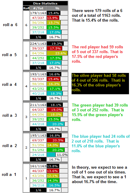
When we are just looking at small numbers of trials just about anything can happen. That is what makes a game uncertain. For example, I have been known to play a version of Risk on a site called GamesByEmail.com. As part of that game, players roll dice to see the outcome of battles. The web site actually keeps track of the rolls and is willing to report the summary if you want it. Figure 5 shows an annotated version of part of that summary for a single game.

Figure 5

One interesting part of examining the summary in Figure 5 is that the players did experience different frequencies of rolling any one particular value, but everyone was close to the expected frequency, namely, 16.7%. The olive player was clearly "lucky" in getting more than her share of the 5's, but that is just the luck of the roll. Had the game gone on longer we would expect the observed values to settle down to the true 16.7% value.

Earlier we looked at an example of having an urn in which we place items of three different colors, mix the items, and then randomly select an item from the urn. The probability of selecting an item of a particular color was simply the ratio of the number of items of that color to the number of items in the urn. Let us carry that concept a bit further.

All of the probability examples that we have seen thus far have been examples of discrete probabilities. When we flip a coin there are two discrete outcomes, heads or tails, and we assign probabilities to each. When we roll a die there are six discrete outcomes, values one through six, and we assign probabilities to each. When we have a container (an "urn") of items identified by nine different characteristics we assign a probability to randomly selecting an item showing each of those characteristics.

Let us consider another discrete case, this one with a slight twist. Our physical model of the situation is to have a container holding many objects. Each object is the same size, shape, and weight. They are distinguishable only in their surface color and design. We will assume each item is just a ball although the actual shape is of no real concern. Each ball has a background color, one of the colors red, blue, yellow, green, and purple. Each ball has a design on it, one of the shapes stars, dots, crescents, and triangles. The items in the container are thoroughly mixed. We will randomly select an item from the container (i.e., blindly reach in and pull one out and examine it). We want to be able to talk about the probability of getting an outcome such as P(x is blue), or P(X has stars), or P(X is red and X has triangles), or P(X is green and X has dots), and so on.

To quantify this situation consider the example shown in Table 3.


Table 3 is also helpful in illustrating another topic, conditional probability. Rather than paging back to look at Table 3 we can restate it here:

Table 3 was constructed with some random values. It was not constructed to be sure that there would be a difference between the conditional probability and the overall probability in the case illustrated above. However, I could construct a table made up of rows called Rj and columns called Ci where it is the case that for a value i and a value j we have
P( Ci | Rj ) = P( Ci )
That condition has a special name. If that condition holds then we say that column Ci is independent of row Rj. In English, to say that
P( Ci | Rj ) = P( Ci )
is just saying that telling us that the item is in row Rj does not help us make a better guess about whether or not the item is in column ci. Perhaps a new table will help illustrate this point.


In fact, Table 4 is made up of independent rows and columns. Feel free to check out any combination.

It is important to note that statistical independence has no meaning beyond that given above. To say that event A is independent of B is just a statement that the probability of event A does not change if we know that B is true. Statistical independence says absolutely nothing about the concept of "cause and effect". This is true even though we fall into the sloppy use of the term dependent when we say that events that are not independent are called dependent. If A is not independent of B then we say A is dependent upon B. This does not mean that B causes or determines A. It just means that if we know that B is true then we need to adjust the probability that A is true.

For the most part we have been looking at sampling with replacement. Sampling without replacement can make our computations much more difficult. For example, consider the case of a container of M&M's. We happen to know the number of pieces of each color in the container. Table 5 gives us those colors. Clearly this situation where drawing items without replacement has a small effect on the probability of selecting the next item is related to both the size of the population, i.e., the number of candies in the container at the start, and to the number of items we are drawing out of the container. If we start with just a few candies then the probabilities will change dramatically. If we sample too many candies the probabilities will change dramatically. The sweet spot here is to have a large population and a relatively small sample. There is a general "Rule of Thumb" related to this that says "If we are sampling less than 5% of the population, then we can overlook the changes in the probabilities and just use the initial probabilities in our computations." Later in this course we will hear that rule again and again as it is applied (sometimes with additional restrictions) to different situations. Even at this first introduction to the rule please note that to say that we are sampling less than 5% of the population is the same as saying that the population is more than 20 times larger than the size of the sample.

Return to Topics page

©Roger M. Palay     Saline, MI 48176     December, 2015