Permutations

Return to Topics page
Permutations are different ways to arrange some group of things. The key concept is that the order of the things in these arrangements is important. If we start with three things, A, B, and C then we can arrange them in any of the following ways: ABC, ACB, BAC, BCA, CAB, or CBA. These are all permutations of the letters A, B, and C. There are 6 permutations of the three things.

Another example would be to start with four things, say, cat, dog, eel, and fox, and ask for the permutations of these four things taken two at a time. That is, find all the different arrangements of two things where the two things are taken from the list of the four things: cat, dog, eel, and fox. This will be cat dog, cat eel, cat fox, dog cat, dog eel, dog fox, eel cat, eel dog, eel fox, fox cat, fox dog, and fox eel. There are 12 permutations of four things taken two at a time.

Clearly there are two related but different tasks here. One is to be able to construct the different permutations and the other is to predict the number of permutations that we will find. R can help us with both of these. Unfortunately, that help will take a little bit of extra effort.

This next section presents the "permutations" function. Although it is nice to see it, this class does not require you to use it. For this class we will get a smaller, easier to use function, in fact we will get two of them, to mimic the function available on the TI-83/84 calculators. Those functions are presented later on this page.

Bill Venables, and later Gregory R. Warnes, developed and refined a special function that constructs permutations. That function is not part of the base R installation. Instead, that function is provided in a package that is called "gtools". In order for us to use that function we must do two things. First we need to actually get the package and second we need to load it into our R session. Fortunately the commands to do both of these are quite short. 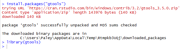They are

install.packages("gtools")
library(gtools)

Once we have performed those two statements within our session we will be able to use the permutations() function. Figure 1 shows the console screen that reflects doing those two commands.

Figure 1

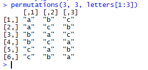
Following the installation shown in Figure 1 we can give the command permutations(3, 3, letters[1:3]) which is a call to the permutations() function, telling it that it should use the 3 values in the third argument and to use them 3 at a time to form all of the possible permutations that it can. The third argument, letters[1:3] provides the letters "a", "b", and "c" for permutations() to use as the values. Figure 2 shows the result of that command.

Figure 2

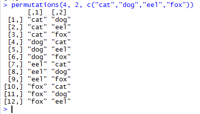
It is always nice to get a confirmation like that. We can try to confirm the "cat dog eel fox" challenge from earlier. The command permutations(4, 2, c("cat","dog","eel","fox")) should do it.

Figure 3

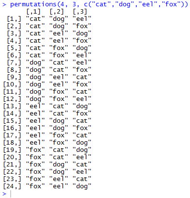
We can make that challenge a bit more difficult if we ask for all the permutations of the 4 things taken 3 at a time by using the command permutations(4, 3, c("cat","dog","eel","fox")) as shown in Figure 4.

Figure 4

As a by-product of having R construct the various permutations we also discover the number of permutations. After all, it really does not matter what values we are using the number of permutations of 3 things taken 3 at a time is 6 (as seen in Figure 2), the number of permutations of 4 things taken 2 at a time is 12 (as seen in Figure 3), and the number of permutations of 4 things taken 3 at a time is 24 (as seen in Figure 4).

Remember that we get the output that we saw in those figures because we just use the function permutations() as a statement. We did not assign the results of the function call to any variable. We will change that behavior with the command t<-permutations(3,3,c("M","A","T","H","1","6","0")) shown in Figure 5.

Figure 5

In Figure 5 the result of the permutations() function is stored in the variable t; the result is not displayed in the console.

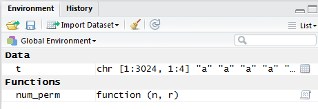
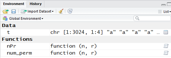
Because the work shown above was done in RStudio, we can find the variable t in the Environment pane. There we see the "dimensions" of t as well as the first few values stored in that variable. This is shown in Figure 6.

Figure 6

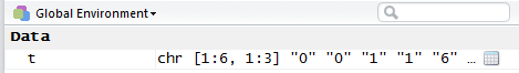
The dimensions [1:6, 1:3] specify that t is structured as 6 rows (numbered 1 through 6) and 3 columns (numbered 1 through 3). This is exactly what we expect since there are 6 permutations each holding 3 values. We could issue the command t to have R display the contents of t. That is done in Figure 7.

Figure 7

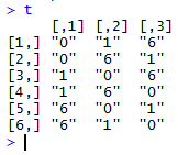
The display in Figure 7 shows our 6 rows and 3 columns. Each row contains a different permutation.

What might be surprising is the values from the third argument, "M","A","T","H","1","6","0", that permutations() seems to have chosen. It almost looks like the function took the last three values instead of the first three that most people would have expected!

In fact, permutations() selected the lexicographically lowest three values. We can see this if we rerun the command but change the choice of values as is shown in Figure 8.

Figure 8

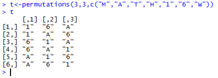
The values shown in Figure 8 are the three lexicographically ordered values in the third argument of permutations(3,3,c("M","A","T","H","1","6","W")). Lexicographic ordering is an extension of what we would call alphabetic ordering. The extension means that we are using the coded values of the characters to sort them. In this case it is enough to point out that the character "1" has a lower "lexicographic" value than does the character "6" which in turn has a lower "lexicographic" value than does the character "A".

One issue with permutations is that it does not take much to create a situation where the number of permutations gets to be quite large. For example, if we use all seven of the characters in MATH160 and ask for the permutations of 7 things taken 3 at a time, we will get 210 permutations. We can see this by running the command t<-permutations(7,3,c("M","A","T","H","1","6","0")) as shown in Figure 9.

Figure 9

Because the functional value was assigned to a variable, t, there is no associated output. However, the information about t displayed in the Environment pane now reflects the new contents of t. Figure 10 shows this diagnostic information.

Figure 10

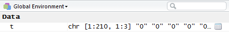
Indeed, the dimensions of t shown in Figure 10 indicate that there are 210 permutations of 7 things taken 3 at a time. Thus, using the diagnostic information in the Environment pane we have found a way to determine the number of permutations that we have for whatever number of things we have taken some number of things at a time. However, we would like to have a more direct way to find that number.

You might notice that when we ask for the number of arrangements of 7 things taken 3 at a time we are really saying that we have three positions to fill using the 7 values, We can form a picture to helps us. Figure 11 shows our three positions and gives them the names first, second, and third.

Figure 11

Then our process is to fill the three positions with the 7 values. We start by filling the first position. We have any of seven choices that we could put into that first position. Once we have made that choice, however, there are only six remaining values that we could put into the second position. That means that there are 7*6 or 42 different ways to just fill the first and second positions. But for each of those 42 arrangements there are still five possible choices for the third position. Therefore, we have 7*6*5 ways to fill all three positions using our 7 possible values. But, 7*6*5=210, the number of permutations of 7 things taken 3 at a time.

This suggests an algorithm for finding the number of permutations of n things taken r at a time. We just form the product of r factors, starting with n and decreasing by one for each new factor. This algorithm says that the number of permutations of 9 things taken 4 at a time is equal to the value of the four factor expression 9*8*7*6, or 3024. Before we go any further we will use our sneaky trick to see if we get the same answer. Figure 12 shows the command to create, but not display, the permutations.

Figure 12

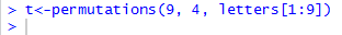
And, Figure 13 shows the dimensions of the new variable t, confirming our answer of 3024.

Figure 13

Here is where we develop our own functions for finding the number of permutations of n things taken r at a time.

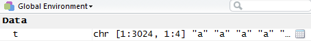
The algorithm of creating the product of r factors, starting with n and decreasing by one for each new factor, can be written in R to define a new function as:

num_perm <- function( n, r )  # compute the number of permutations
{                             # of n things taken r at aa time
  if( r == 0 )                #  special case if r=0
    {return(1)}
  p <- 1                      # initialize the product
  for (i in 1:r)              # go throgh the r factors
  { p <- p*n
    n <- n-1
  }
  return(p)                   # send back the result
}

When this text is given to R it just accepts the definition as shown in Figure 14.

Figure 14

The first confirmation of the acceptability of our new function is that R did not complain about any errors. The second confirmation is that the new function, num_perm() is now shown in the Environment pane shown in Figure 15.

Figure 15

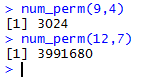
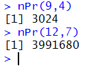
Once our new function is defined we can run it by using its name and sending it two values. For example we can have it find the number of permutations of 9 things taken 4 at a time by giving the command num_perm(9,4). R responds with our much anticipated 3024. Or we could have our function find the number of permutations of 12 things taken 7 at a time by giving the command num_perm(12,7). In that case R responds with 3991680. All of this is shown in Figure 16.

Figure 16

In all of the discussion above we have written out the challenge in the form "find the number of permutations of n things taken r at a time." It would be nice if we has some way to say this in just a few symbols. Unfortunately, there has not been any agreement on the most acceptable form for such symbolism. One form _nP_r has a small advantage in that it is the form used by the TI-83/84 calculators. On such a calculator one would enter 12_nP_r7 to find the number of permutations of 12 things taken 7 at a time. However, in a textbook or paper, the symbol for that specific computation would be ₁₂P₇. Table 1 gives some the general and specific forms.

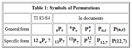
Here we will try to consistently use the _nP_r form.

Now that we have a symbol for permutations, it would be nice to have a direct way to express the formula without having to print out our function. The first step in doing this is to note that ₆P₆ = 6*5*4*3*2*1. In fact, _nP_n = n*(n-1)*(n-2)*...*3*2*1. We have a mathematical symbol for 6*5*4*3*2*1 and that is 6! which is read as "6 factorial." That means that 8! = 8*7*6*5*4*3*2*1 and n! = n*(n-1)*(n-2)*...*3*2*1.

It would be nice if we were able to use the factorial symbol to help write the equation for permutations. However, ₈P₃ = 8*7*6; it only has three factors. We need to find a way to say that we should stop appending factors at some point. The general form _nP_r will have r factors. It could be written as _nP_r = n*(n-1)*(n-2)*...*(n-r+2)*(n-r+1). That is, the general form says that we start the factors at n but stop when we get to the factor equal to (n-r+1). We can verify that for n=8 and r=3 which makes (n-r+1) be 6 and, indeed, our factors start at 8 and end at 6 to get 8*7*6.

Unfortunately, there is no symbolic way to say "Start doing 8 factorial but stop after 3 factors are in place." However, we can observe that

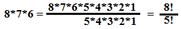This pattern gives us a way to write, in a short space, the value of the product of three numbers starting at 8 and decreasing by 1 each time. We know that ₁₂P₅ = 12*11*10*9*8 but we could write that as ₁₂P₅ = (12!) / 7!. In general terms we state this pattern as

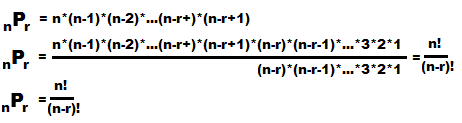This formula, _nP_r = n! / (n-r)!, is the one generally quoted as the way to find the number of permutations of n things taken r at a time. The formula works and if we have some way to find factorials then this becomes a convenient formula.

Back in Figure 14 we saw a function that we wrote, num_perm(). That function did not use factorials at all. It turns out that R has a built-in function, factorial() that computes factorials. Therefore, we could, if we wanted to, create a new function that does the same thing that the old one did but this time uses factorial(). One possibility for this would be

nPr <- function( n,r )
{ return (factorial(n)/factorial(n-r))}

Figure 17 shows this function definition in RStudio session.

Figure 17

We can see, in the Environment pane shown in Figure 18, that R has accepted the function definition.

Figure 18

Now that the function is defined we can use it by entering commands such as nPr(9,4) or nPr(12,7) as demonstrated in Figure 19.

Figure 19

Of course we got the same results as we did from num_perm() back in Figure 16.

Now we have two functions, num_perm() and nPr(), that do the same thing. Which should we use? It really does not make a difference; we get the same answer with either function. Use whichever appeals to you.

Before we leave this topic there is one sticky point that we need to cover. The factorial() function makes sense for things like factorial(9) or factorial(3). It even makes some sense that factorial(1) gives the answer of 1. However, look at Figure 20.

Figure 20

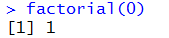
According to Figure 20, 0! is 1. On the surface this may seem strange but it a a part of the definition of factorial. In fact, we need 0! to be defined to be 1 so that our formula for the number of permutations works out in the extreme cases. We already know that the number of permutations of 6 things taken 6 at a time is the same as 6!. But our formula says that ₆P₆ = 6! / (6-6)!. Simplifying that denominator means that ₆P₆ = 6! / 0!, so we need to define 0! to be 1.

Return to Topics page
©Roger M. Palay Saline, MI 48176 December, 2015