Combinations
Return to Topics page
Combinations are different ways of selecting items from a group.
The key concept is that the order of the chosen items is not important.
If we have four things, A, B, C, and D, then we can select
two items in any one of six ways, AB, AC, AD, BC, BD, and CD.
Because order is not important, the choice DA is already in our list of
six in the form AD.
Another example would be to start with five things, say
cat, dog, eel, fox, and goat.
Then we could ask for the combinations of those five things
taken three at a time.
That is, find the different groups of three things that we can make using just the
five things cat, dog, eel, fox, and goat.
That will be the 10 groups
1:cat dog eel, 2: cat dog fox, 3:cat dog goat
, 4:cat eel fox, 5:cat eel goat,
6:cat fox goat, 7:dog eel fox, 8:dog eel goat
, 9:dog fox goat, and 10:eel fox goat.
Thus, there are 10 combinations of 5 things taken 3 at a time.
We note that the group fox cat eel is already in the answer as
cat eel fox because the order of items in the group is not important.
Clearly there are two related but different tasks
here. One is to be able to construct the different combinations and the other is
to predict the number of combinations that we will find.
R can help us with both of these.
Unfortunately, that help will take a little bit of extra effort (this effort
is the same as that done for permutations and it need not be repeated if
it was already done in our RStudio or R session).
| This next section presents the "combinations" function. Although it is nice to see it,
this class does not require you to use it. For this class we will
get a smaller, easier to use function, in fact we will get two of them,
to mimic the function available on the TI-83/84 calculators. Those functions are presented
later on this page.
|
Bill Venables, and later Gregory R. Warnes, developed and refined
a special function that constructs combinations. That function
is not part of the base R installation. Instead, that function is
provided in a package that is called "gtools". In order for us to use that
function we must do two things. First we need to actually get the package
and second we need to load it into our R session.
Fortunately the commands to do both of these are quite short.
They are
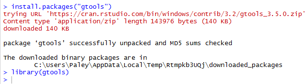
install.packages("gtools")
library(gtools)
Once we have performed those two statements within our session we will be able to use the
combinations() function. Figure 1 shows the console screen
that reflects doing those two commands.
Figure 1
Following the installation shown in Figure 1 we can give the command
combinations(4, 2, letters[1:4]) which is a call to the
combinations() function, telling it that it should use
the 4 values in the third argument and to use them 2 at a time
to form all of the possible combinations that it can. The third argument,
letters[1:4] provides the letters "a", "b", "c" and "d" for combinations()
to use as the values.
Figure 2 shows the result of that command.
Figure 2
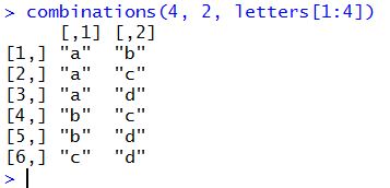
That is the same result, but with lower case letters, that we saw in the
example used at the top of the page. We can do the second example, the
one looking at the combinations of cat, dog, eel, fox, and goat
taken 3 at a time via the command
combinations(5,3,c("cat","dog","eel","fox","goat")).
This is shown in Figure 3.
Figure 3
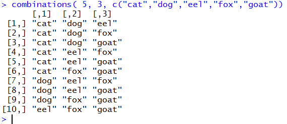
It should be clear from Figure 2 and Figure 3 that we could use the R
function combinations() to not only produce the possible combinations
but also to find the number of such combinations.
Before we go any further, we should pause for a moment and
find some way to symbolize "the number of of combinations
of n things take r at a time."
As was the case with permutations there are many such symbols.
Unfortunately, there has not been any
agreement on the most acceptable form for such symbolism.
One form nCr has a small advantage
in that it is the form used by the TI-83/84 calculators.
On such a calculator one would enter 12nCr7
to find the number of combinations of 12 things taken 7 at a time.
However, in a textbook or paper, the symbol
for that specific computation would be 12C7.
Table 1 gives some the general and specific forms
of the ways we put "the number of of combinations
of n things take r at a time" into symbols.
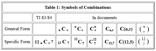
The final form in Table 1,  ,
is often seen in math classes, but
here we will try to consistently use the general form nCr,
or in specific problems the 12C7 form.
,
is often seen in math classes, but
here we will try to consistently use the general form nCr,
or in specific problems the 12C7 form.
The combinations of taking 5 things, 3 at a time were illustrated above
in Figure 3.
There we found that there were 10 such combinations.
Each of those combinations has 3 things in it.
We recall that the number of permutations
of 3 things taken 3 at a time is
3! = 3*2*1 = 6.
In our earlier example, one of the combinations was
cat eel goat.
But this could be arranged as
1:cat eel goat,
2:cat goat eel,
3:eel cat goat,
4:eel goat cat,
5:goat cat eel, or
6:goat eel cat.
Therefore, each of the 10 groups representing a different
combination of 3 things taken from the original 5 things
could be arranged in 6 ways.
If we did that then we would have the 60 permutations
of 5 things taken 3 at a time,
5P3 = 5! / (5-3)! = 5! / 2! = 5*4*3 = 60 =10*6 = 5C3*3P3.
That is, 5P3 is equal to
5C3 times 3P3.
There is no trick here as concerns the numbers we are using. It is always the case that
nPr = nCr * rPr
Of course we can solve that equation for nCr
to get
nCr = nPr / rPr
This formula is all we need to construct a function
in R to compute the number of
combinations of n things taken r
at a time.
|
Here is where we develop our own functions
for finding the number of
combinations of n things taken r at a time.
|
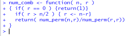
The code for such a function is
num_comb <- function( n, r )
{ if( r == 0 ) {return(1)}
  if( r > n/2 ) { r <- n-r}
  return( num_perm(n,r)/num_perm(r,r))
}
and Figure 4 shows that function entered into an R session.
Figure 4
We note that R accepted the form of the function
in that Rgave no error message at this point.
A second confirmation of this is that the function is
now defined in the environment pane
of our RStudio session.
Figure 5
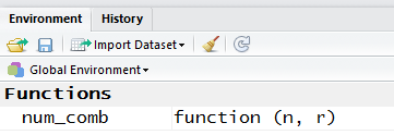
Even though there was no error in the way we wrote num_comb(),
examining the Environment pane in Figure 5 reveals
that the function num_comb() will not work in this
R session. It will not work because we wrote the function
to use another funcion, namely, num_perm(), and that
function has not been defined in this session.
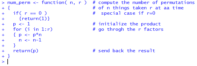
To fix this problem we will have to define num_perm().
This is shown in Figure 6.
Figure 6
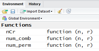
We revisit the Environment pane and now both functions are defined.
Figure 7
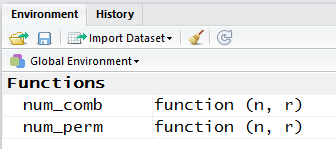
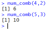
Figure 7 shows two example calls to the num_comb() function.
The first asks for the number of combinations of 4
things taken 2 at a time.
The second asks for the number of combinations of 5
things taken 3 at a time.
We already knew these answers from Figure 2 and Figure 3, respectively.
Figure 8
In Figure 9 we look at all the other possible requests
for combinations involving 5 things.
Figure 9
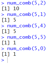
The results shown in Figure 9 are worth some examination and consideration.
In the first place, 5C2 is 10,
exactly the same value that we had for
5C3.
This is not a coincidence!
If we have 5 items, say A, B, C, D, and E,
and we select 3 of them, perhaps A C D,
then there are exactly 2 that we did not select;
in our example that would be B E. In fact, each time we select
3 items for 5C3 the 2 items
not selected will be one of the combinations
that make up 5C2.
This same pattern is shown in
comparing 5C1
and 5C4.
Each time we select
1 item for 5C1 the 4 items
not selected will be one of the combinations
that make up 5C4.
In general, it is always true that
nCr = nC(n-r).
We actually used that fact in the
definition of num_comb()
when we included if( r > n/2 ) { r <- n-r}
That line means that if we ask for num_comb(12,9) then
the function really computes num_comb(12,3). We
did this because it makes the computation shorter. Both num_perm(12,9)
and num_perm(9,9) have 9 factors.
However, each of num_perm(12,3)
and num_perm(3,3) have only 3 factors.
The second thing to note from Figure 9 is that
5C0 is 1.
This does raise the question of what it means to have
5 things and take them 0 at a time? We can answer that
by following the same pattern that we just saw in understanding why
5C3 = 5C2.
Our understanding of that is that each combination of 3 things
taken fom our 5 things leaves a combination of 2 things.
Using that pattern we know that
5C5 = 5C0.
Our understanding is that each combination of 5 things
taken fom our 5 things leaves a combination of 0 things.
But our combination of 5 things is all of them and that leaves
the empty set as as the one and only combination of 0 of the original 5.
Therefore, 5C0 is 1.
A third thing to note from Figure 9 (and Figure 8) is that if we look at
the values in the following order
5C0,
5C1,
5C2,
5C3,
5C4, and
5C5, then we get
1 5 10 10 5 1.
That is exactly row 5 of Pascal's Triangle, the top of which is shown in Figure 10.
Figure 10
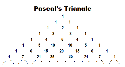
Each row of the triangle starts with and ends with a 1.
Internal values in a row are just the sum of the two values in the previous
row that are above and to the left and right of the position of that internal number.
Thus, in row 6 (the top row is row 0),
the value 15 is just the sum of the 5 and 10 in row 5.
Pascal's Triangle gives us the "binomial coefficients" for the expansion of an
expression such as (x+y)5. Thus,
(x+y)5 = 1x5y0 +
5x4y1 +
10x3y2 +
10x2y3 +
5x1y4 +
1x0y5
Leading up to the development of the num_comb() function above, we had
nCr = nPr / rPr
But we already have a formula for permutations so we know that
nPr = n! / (n-r)! and
rPr = r! / (r-r)! = r! / 0! = r! =r!
Therefore, we could rewrite our equation for combinations as
nCr = ( n! / (n-r)! ) / (r!)
This is mathematically equivalent to
nCr = n! / ( (n-r)! * r! )
This is the usual statement of the formula for the
number of combinations of n things taken r at a time,
although it is most often written in a more conventional fraction form as
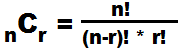
This allows us to construct a new function to
compute nCr, but this time without having to
make reference to the num_perm() function.
The code for the new function is
nCr <- function(n,r )
{ return ( factorial(n)/factorial(n-r)/factorial(r))}
and Figure 11 shows the function as entered into an RStudio session.
Figure 11

Checking the Environment pane shows the new function.
Figure 12
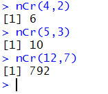
And, finally, we can use the statements nCr(4,2),
nCr(5,3), and nCr(12,7) to test out the new function,
as shown in Figure 13.
Figure 13
Return to Topics page
©Roger M. Palay
Saline, MI 48176 December, 2015