Confidence Interval for the population mean, μ,
based on the sample mean when
σ is unknown
Return to Topics page
Review:
The concept of a confidence interval
was developed on a previous page.
There we saw that we can take the sample mean,
 ,
as a point estimate
of a population mean, and form an interval with the
point estimate as the center of the interval
and the lower and upper ends of the interval set at
a distance, called the margin of error, on
either side of the point estimate.
Furthermore, we used the fact that the
distribution of sample means is normal
to help us determine the value of the margin of error.
,
as a point estimate
of a population mean, and form an interval with the
point estimate as the center of the interval
and the lower and upper ends of the interval set at
a distance, called the margin of error, on
either side of the point estimate.
Furthermore, we used the fact that the
distribution of sample means is normal
to help us determine the value of the margin of error.
Part of that determination was to state the level of confidence
that we want in the process. Thus, we create a 95% confidence interval
by a process that will generate confidence intervals wide enough
so that 95% of the confidence intervals generated by this
process will contain the true population mean, μ.
To do this we used that the fact that the distribution of the sample mean
is not only normal but it has a mean of μ and
a standard deviation = .
That meant that for a 95% confidence interval we needed
to find a z-score,
.
That meant that for a 95% confidence interval we needed
to find a z-score,  ,
such that 95% of the area under the
standard normal curve is between the z-score and its negative.
Once we have the z-score then the margin of error is just
,
such that 95% of the area under the
standard normal curve is between the z-score and its negative.
Once we have the z-score then the margin of error is just
 and the confidence
interval
and the confidence
interval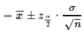 .
.
New:
That whole process depends upon us knowing the value of σ,
the population standard deviation.
I hope that you can see how unlikely this is.
The whole process is designed to find a confidence interval
for the population mean. It would be absurd to do this if we already
know the population mean.
The process above requires that we know the population standard deviation.
Since the population standard deviation is the
root mean squared deviation from the mean, we need to
know the population mean in order to compute the
population standard deviation.
It does raise the question of why we developed a process that we will never use?
We introduce the process above because it is a great model for
creating a confidence interval when the population standard
deviation is unknown.
In such a situation we use the sample standard
deviation, sx,
as a approximation to the population standard deviation.
When we do this can no longer compute the standard deviation of the
sample mean by because we do not
know σ. Instead, we compute the standard deviation of the sample mean
by  .
However, computed this way, we cannot
say that the sample mean
is N(μ,sx),
instead we say that the sample mean has a Student's t distribution
with n-1 degrees of freedom.
Knowing this we can just mimic the earlier process, substituting
the use of the Student's t with the appropriate
degrees of freedom for our
value.
.
However, computed this way, we cannot
say that the sample mean
is N(μ,sx),
instead we say that the sample mean has a Student's t distribution
with n-1 degrees of freedom.
Knowing this we can just mimic the earlier process, substituting
the use of the Student's t with the appropriate
degrees of freedom for our
value.
From a sample of size n=25 with a sample
mean =134
and sx=6,
to find a 95% confidence interval
we look at the Student's t distribution for
25-1 = 24 degrees of freedom
to find the t-score such that the area under
the curve between that t-score and its opposite
is 0.95 square units, (95% of the area). To do this we could
look at the 24 degrees of freedom table
to find the value that has 0.025 to its left.
The portion of that chart that we would use is shown
in Figure 1.
Figure 1
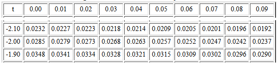
The t-score -2.06 has 0.0252 square units to its left.
The t-score -2.07 has 0.0247 square units to its left.
We want to move 0.0002 of the 0.0005 square unit difference,
that is, 2/5 of the way.
Therefore, by interpolation, our best guess at the answer is
-2.064.
Or, because we want the convenient 0.025 area to the left
of the t-score, we could use the
Critical Values of the Student's t
table. The portion of that chart that we would use is shown in
Figure 2.
Figure 2
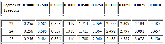
There, on the row for 24 degrees of freedom
and in the 0.0250 column, we find that the
t-score 2.064 has 0.025 square units to its right.
Note that this time we found the positive part of the pair
of t-scores.
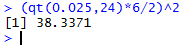
Or, because we can use R, we could just give either
one of the two commands qt(0.025,24) or
qt(0.025,24,lower.tail=FALSE), to find the
t-score with 0.025 to the left or the
t-score with 0.025 to the right, respectively.
Figure 3 shows the commands and the results.
Figure 3
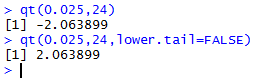
It makes no difference if we find the positive
or the negative t-score.
The margin of error will be
m and the absolute value means that the sign of the
t-score does not make a difference in the result.
When we compute the confidence interval the
formula is
and the absolute value means that the sign of the
t-score does not make a difference in the result.
When we compute the confidence interval the
formula is  and the ± means that the sign of the t-score
will not make a difference.
and the ± means that the sign of the t-score
will not make a difference.
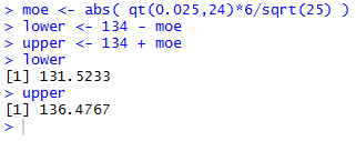
For the problem we have been using, n=25,
=134, sx=6,
find a 95% confidence interval, the calculation of the
margin of error and the resulting lower
and upper endpoints of the
confidence interval are shown
in Figure 4.
Figure 4
Just as we saw in the case where we know the population standard deviation,
we can change the magnitude of the margin of error in
two ways. First, if we increase the level of confidence
then the resulting confidence interval will be wider so that
more of the samples produced using this process will include the
true population mean. Alternatively, if we
decrease the level of confidence then the resulting
confidence interval will be narrower because
we can have more of the intervals produced by this process miss the true
population mean.
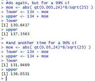
To illustrate this, we could do the same computations
but for a 99% confidence interval (should be wider)
and a 90% confidence interval (should be narrower).
These are done in Figure 5.
Figure 5
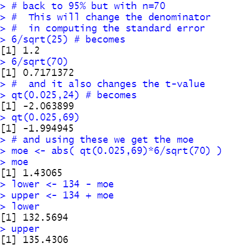
The second way we can alter the width of the confidence interval
is by changing the sample size. The larger the sample size
the larger is the denominator in the formula for the
margin of error resulting in a smaller value.
If we return to the original problem, the 95% confidence interval
but we increase the sample size to 70 then
we will find that the resulting confidence interval
will be narrower.
That computation is shown in Figure 6.
Figure 6
If we have a desired margin of error, m,
then we can use a little algebra to change
m=
into 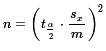 to create a formula for determining the
required sample size, n, once we have set the
confidence level and we have a good idea about the
eventual magnitude of sx.
Note that each time we take a sample we will get a different
sx but those values should not
wonder around too much, especially for larger values of n.
Thus, although we can get a good idea of the required
sample size, we cannot get the exact value
that we were able to get in the case where we knew the
population standard deviation.
to create a formula for determining the
required sample size, n, once we have set the
confidence level and we have a good idea about the
eventual magnitude of sx.
Note that each time we take a sample we will get a different
sx but those values should not
wonder around too much, especially for larger values of n.
Thus, although we can get a good idea of the required
sample size, we cannot get the exact value
that we were able to get in the case where we knew the
population standard deviation.
For the current example,
where have a sample size of 25,
we found a margin of error
of about 2.4767. We could compute
the sample size needed to get that down to 2.00 as shown in Figure 7.
Figure 7
That computation suggests that a sample size of 39
will be large enough to accomplish our goal.
However, when we draw a sample of size 39 there is no
way to be sure that the sample standard deviation,
sx, will stay at 6.
This would be a good time to return to the web page that
takes 1000 samples of a given size and computes confidence intervals
for each sample.
The starting web page is
Set Parameters.
Figure 8 shows the initial screen settings on that page.
Figure 8
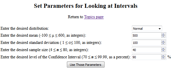
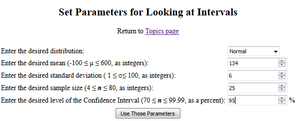
We can change those values so that we are looking at a
normal population with μ=134 and σ=6.
Then we specify that we want samples of size 25 and
we want to see 95% confidence intervals.
Now the page appears as in Figure 9.
Figure 9
At that point if we click on "Use Those Parameters" then
we get a new page with a population, 1000 samples, and
confidence intervals for each. Furthermore, each that
you return to that page and click the button you get a new population
and new samples. I clicked on the button and got a new page that I then saved
so that it would be available, as a static page, for us to review.
The page is at Saved Example.
That page starts with a confirmation of the
desired population parameters and the listing of the population
values. Figure 10 shows the parameters and
first 20 values.
Figure 10
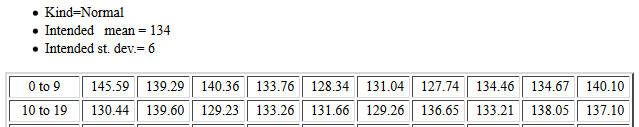
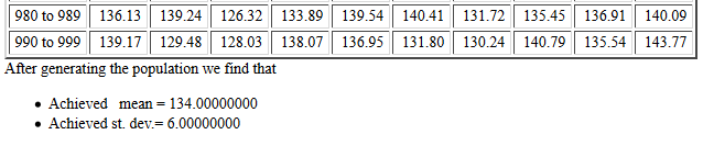
Figure 11 shows the end of the population values
and a statement that we
indeed have met the expectations.
Figure 11
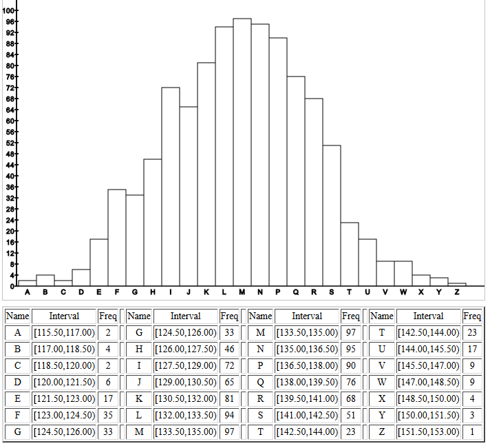
The histogram of the population confirms the
normal distribution characteristic.
Figure 12
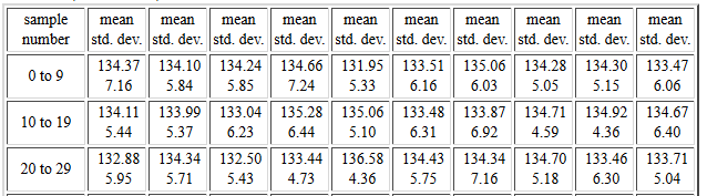
Then, in Figure 13, we see mean and standard
deviation of the first 30 of the 1000
samples, each of size 25.
Figure 13
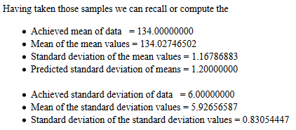
After the listing of the 1000 samples,
we find in Figure 14 that the report on the samples.
One thing to note here is how close the actual
standard deviation of the sample means
is to the predicted value.
Figure 14
The histogram of the 1000 sample means confirms the
normal distribution of the sample means.
Figure 15
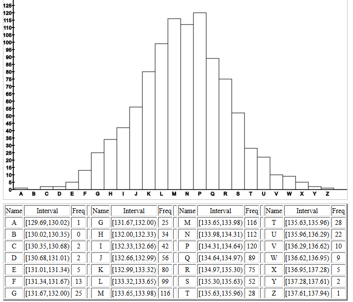
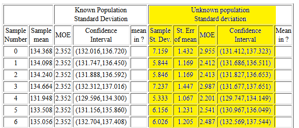
Figure 16 shows the start of the
listing of the 95% confidence intervals
that are generated for each of the samples.
The left columns show the construction of the
confidence interval based on the known population
standard deviation.
The highlighted right columns show the construction
of the confidence intervals based on the
sample standard deviation and
the Student's t distribution.
Remember that the
confidence level is set to 95% and that
the degrees of freedom is 24.
For each sample the table shows the sample mean in the second column,
the sample standard deviation in the sixth column,
the standard error, which is the sample standard deviation
divided by the square root of the sample size,
in the seventh column, the margin of error in the eighth column,
and the confidence interval in the ninth column.
Figure 16
There is a lot to learn from the information
in that table. First, unlike the confidence intervals on the left
where the margin of error is always the same, each of the
confidence intervals on the right have different values for the margin
of error.
Second, the values for the margin of error on the right
can be smaller or larger than the uniform value in the left portion.
This is true even though the value
of tα/2≈-2.064
which is larger than the value of
zα/2≈-1.96.
This is because the sample standard deviation,
sx can be much less than the
population standard deviation, σ.
For example, look at sample number 4. There the sample
standard deviation is 5.333, much less than the
population standard deviation, 6.
Third, even though the confidence
interval on the right can be smaller,
in each of the cases shown in Figure 16,
both the left and the right confidence
intervals contain the true population mean.
Remember that we have
constructed 95% confidence intervals
and therefore we only expect 5%
of the intervals that we generate to miss the true population mean.
We will have to look down the table to find such examples.
Samples 453 through 458 contain such examples.
That part of the table is shown in
Figure 17.
Figure 17
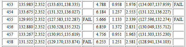
For sample #453, if we know the value of σ we
generate the left confidence interval and it does contain the true mean.
However, sample #453 has a small standard deviation and that,
combined with a really high sample mean,
gives rise to a narrow confidence interval that
does not contain the true mean. That is why the table holds
FAIL in the tenth column.
In sample #455 the sample mean is so low that both
confidence intervals miss the true μ.
In sample #458 the sample standard deviation is so large that
even though the sample has a low mean, the confidence interval
constructed using sx still contains
μ whereas the confidence interval constructed using σ
does not.
At the end of the table of confidence intervals the web page
provides the information shown in Figure 18.
Figure 18
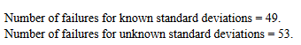
From that we learn that 49 of the 1000 confidence intervals
generated using σ and the appropriate z-score
failed to contain μ. Not bad considering we expect
to fail 5% of the 1000 times.
We also learn that 53 of the 1000 confidence intervals
generated using sx and the
appropriate t-score
failed to contain μ.
Again, not bad considering that we expect
to fail 5% of the 1000 times.
Automating the process
The process of computing a confidence interval
in the case where we do not know the
population standard deviation and where
we have a sample of size n that yields a
sample mean  and a sample standard deviation sx is
as follows:
and a sample standard deviation sx is
as follows:
- From the confidence level compute the
value of
 using
using

- Use qt()
to find the associated t-score,
tα/2
- Find the margin of error as
- Find the two parts to the confidence interval by evaluating
We should be able to describe these same actions using R
statements inside an R function.
Consider the following function definition:
ci_unknown <- function( s=1, n=30,
                        x_bar=0, cl=0.95)
{
  # try to avoid some common errors
  if( cl <=0 | cl>=1)
  {return("Confidence interval must be strictly between 0.0 and 1")
  }
  if( s < 0 )
  {return("Sample standard deviation must be positive")}
  if( n <= 1 )
  {return("Sample size needs to be more than 1")}
  if( as.integer(n) != n )
  {return("Sample size must be a whole number")}
  # to get here we have some "reasonable" values
  samp_sd <- s/sqrt(n)
  t <- abs( qt( (1-cl)/2, n-1))
  moe <- t*samp_sd
  low_end <- x_bar - moe
  high_end <- x_bar + moe
  result <- c(low_end, high_end, moe, samp_sd)
  names(result)<-c("CI Low","CI High",
                   "MOE", "Std Error")
  return( result )
}
This does all of our tasks, including returning the
confidence interval as well as some other values.
The file of this function is available from
ci_unknown.R.
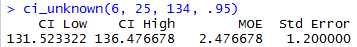
We can try out the new function with
the statement ci_unknown(6, 25, 134, 0.95)
to do the example we solved back in Figure 4. This is shown in
Figure 19.
Figure 19
To reconstruct the confidence interval for
sample #458 shown back in Figure 17
we can use
the statement ci_unknown(6.253, 25, 131.522, 0.95)
as in Figure 20.
Figure 20

Worksheet for a Confidence Interval
Here is a link to a worksheet
with randomly generated problems related to
finding confidence intervals when the standard deviation of the population
is unknown.
Return to Topics page
©Roger M. Palay
Saline, MI 48176 January, 2016