Confidence Interval for Population Mean, μ, based on
the sample mean when σ is known
Return to Topics page
There is a great deal of material to cover before we really get to
confidence intervals.
Fortunately, we have done that work in
previous pages. We summarize that work in Table 1.
| Table 1 |
Probability
- We have discrete and continuous probability distributions.
- For continuous probability distributions we can show a curve of the
probability density function.
- The area under the entire curve is 1.00.
- The area under the curve and to the left of a value v
is the probability that the random variable X is less than v.
This is written as P(X<v).
- For a continuous probability, since there is no "area" under the curve at
a value v, P(X=v) = 0. Therefore,
P(X < v) = P(X ≤ v).
- For symmetric probability distributions we have
P(X < v) = P(X > -v).
- For two values a and b, where a < b,
we have P( a < X < b) = 1 - P(X<a or X>b).
|
The Normal Distribution
- The normal distribution is a continuous probability distribution.
- The normal distribution is based on a mathematical formula.
- The standard normal distribution has mean=0 (μ=0)
and standard deviation=1 (σ=1).
- We have a table to find the area under the standard normal
distribution probability density function curve and to the left of a
value z, i.e., P(X<z).
- We have a function in R called pnorm() to find the
area under the standard normal density function to the left of a
value z, pnorm(z).
- We know how to read the table "backwards" so that if we are given a probability p
we can find the value z that makes P(X<z)=p true.
- We have a function in R called qnorm() that
finds the value z needed to make the P(X<z) be the
value of a specified probability p, that is qnorm(p)
produces the value z so that P(X<z)=p.
- We use N(μ, σ) to symbolize a distribution that is
normal with mean=μ and standard deviation=σ.
- The standard normal distribution is N(0,1).
- We use
 to map a non-standard
normal distribution, N(μ,σ) to N(0,1). to map a non-standard
normal distribution, N(μ,σ) to N(0,1).
- Both pnorm() and qnorm() have extended forms
that allow us to use them directly with non-standard normal distributions.
|
The Sample Mean
- For any original population if we take repeated
samples of size n, with n≥30, with replacement,
then the distribution of the mean of those
samples will be approximately N( μ,σ/sqrt(n) ),
where μ is the mean of the original population and
σ is the standard deviation of the original population.
- If the original population is approximately normal, then the
value of n can be smaller than 30.
|
With all of this, consider the following situation. First, let us find
the z-score in N(0,1) such that P(X<z)=0.025.
We will do this with qnorm(0.025) as shown in Figure 1;
Figure 1
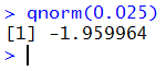
That value is so close to -1.96 that we will use the rounded
value for the rest of this discussion. The meaning of the -1.96
is that for a N(0,1), 2.5% of the area under the curve is to the left of
-1.96.
Since the normal distribution is symmetric, this means that
P(X>1.96)=0.025 also. Thus, 95% of the area is between -1.96
and 1.96. Remember that in our standard normal distribution the
standard deviation is 1. Therefore, we really could have said that 95%
of the area is within 1.96 standard deviations from the mean.
This will be true of any normal distribution.
Now, we
start with a population
that has a known standard deviation, σ. It also has
a known mean, μ. We plan to take a sample of size 36.
We know that the distribution of sample means
from size 36 samples is N(μ,σ/sqrt(36)),
or simplifying, N(μ,σ/6).
If that is the distribution of the means of
size 36 samples, then
we know that 95% of the samples that we take
will have a sample mean that is between
μ-1.96*σ/6 and
μ+1.96*σ/6. This is shown at the top
of Figure 2 where the point a is 1.96 standard deviations
below the mean and point b is 1.96 standard deviations above the mean.
Again, given the distribution of the sample means, if we take
repeated samples of size 36, then 95% of those samples
will have a sample mean that falls between a and b.
Figure 2
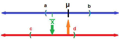
We take our sample. It turns out that our sample mean is
 and, for this part of the discussion, we will assume that it is
one of the 95% of the sample means that falls between a
and b. We see this in Figure 2. Then, on a new line, the lower one in Figure 2,
let us look at the interval that is just as wide as was the one from a
to b. In Figure 2 that interval is from c to d.
and, for this part of the discussion, we will assume that it is
one of the 95% of the sample means that falls between a
and b. We see this in Figure 2. Then, on a new line, the lower one in Figure 2,
let us look at the interval that is just as wide as was the one from a
to b. In Figure 2 that interval is from c to d.
Then, it must be true, if
is in the interval (a,b), then the mean, μ,
must be in the interval (c,d).
Try it again.
Choose any point in (a,b), drop down to the lower line,
then construct a new interval around that value on the lower
line (using the same width interval). The value of the true mean, μ,
will have to be in that new interval.
Similarly, if you choose to put outside of the interval
from a to b (so it is one of the 5% of the sample means that fall outside
of the interval), then it must be the case that the true mean, μ is
not
in that new interval.
This is a spectacular result! It tells us that if we take
a sample of size 36 from a population with a known standard deviation,
let us say it is 12, and if we find that the sample mean turns out to be
43, then we can construct an interval around that value of 43
and make that interval go from
43-1.96*12/6 = 43-1.96*2 = 43-3.92 = 39.08
to
43+1.96*12/6 = 43+1.96*2 = 43+3.92 = 46.92.
We have no way of knowing if the true mean of the population is
in that interval, but we can say that if we follow this same procedure over and over,
95% of the intervals that we would construct will contain the true mean.
This is a 95% confidence interval.
The beauty of this is that we did not need to know the
population mean to do this.
In fact, if we know the population mean then there is no sense in
finding a confidence interval for the population mean.
This procedure is to be used when we do not know the population mean
but we want to
make a good guess as to the value of that mean.
Our best point estimate for the population mean
is the sample mean.
However, the point estimate is almost certainly wrong.
It might be off by a little; it might be off by a
lot, but it is almost always off.
What we want is an interval of values where we can be
relatively certain that our method of creating the interval
tells us that some specified high percentage of the intervals
created this way do in fact hold the
population mean.
The little twist to this is that to use our method we need to know the
population standard deviation.
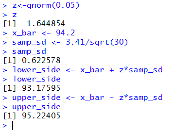
If we know σ, for a new case we say it is 3.41, then
we can choose a level of significance, say 90%.
We calculate the percent we are missing, 100%-90%=10%.
We figure that we need half of that 10% below and half of that above
our interval. In this case we would have 5% below and 5% above.
Since sample means form a normal distribution, we can find
the z-score that has 5% to its left by using qnorm(0.05).
This turns out to be approximately -1.645.
We set the size of the sample;
in this case we will use a sample of size 30.
With the population standard deviation being 3.41,
the standard deviation of the means of samples of size 30 will be
3.41/sqrt(30)≈3.41/5.4772≈0.62258.
We take the sample and find that
=94.2.
Then we construct our 90% confidence interval
by taking ±-1.645*3.41/sqrt(30)
or 94.2±(-1.645*0.62258) or 94.2±-1.02414
or from 93.175859 to 95.22414, which we might express in rounded form as
(93.176,95.224).
These computations are shown in Figure 3.
Figure 3
A few notes on this before we state the general formula,
look at numerous examples, and then look at
automating the process. First, to do this we need to know four things:
the population standard deviation, the sample size, the desired
confidence interval, and finally the sample mean. Second,
by looking at the left tail, asking as we did above for the z-score
such that P(X<z)=0.05, the result stored in x will be
a negative value.
That is why we use addition in
lower_side <- x_bar + z*samp_s.
There are many ways for us to have changed the value
in z to be the positive
side of the pair, and then we would have been able to use a
more sensible subtraction to get the lower_side and an addition
to get the upper_side.
Third, and I wanted to sneak this in where few
people will read it, this type of problem is
at best an academic exercise.
We are supposed to know the population standard
deviation without knowing the population mean. To find the standard deviation
we need to know either the mean for one formula or the sum of the values and the
number of values for the other. Still, we need to do this because it sets the
stage for a more realistic problem, finding the confidence intervals
when we know neither the mean nor the standard deviation of the population
The General Formula
In general, we start with a population, and we know that the
population standard deviation is σ.
We determine a confidence level, cl.
We determine a value we will
call  read as "alpha over 2", which is half the area not in the confidence
interval. Thus,
read as "alpha over 2", which is half the area not in the confidence
interval. Thus,  .
Using we find the
z-score such that P(X < z)=.
We refer to that z-score as
.
Using we find the
z-score such that P(X < z)=.
We refer to that z-score as
 .
We determine a sample size n and take a sample of size n
from which we compute the mean of the sample,
.
At that point we can compute the two ends of the
confidence interval as being
.
We determine a sample size n and take a sample of size n
from which we compute the mean of the sample,
.
At that point we can compute the two ends of the
confidence interval as being 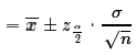 .
.
Please note that  is called the
margin of error. The absolute value sign is there just so that
we always get a positive value for the margin of error.
The width of the confidence interval is always
two times the margin of error.
is called the
margin of error. The absolute value sign is there just so that
we always get a positive value for the margin of error.
The width of the confidence interval is always
two times the margin of error.
We really have two ways that we can change the size
of the margin of error
and, thus, change the width of the confidence interval.
The first is by changing the size of the sample.
The larger we make the sample
size, n, the larger is the denominator in the
margin of error. The larger the denominator, the smaller the
margin of error. Back in Figure 3 we never expressed the
margin of error as a separate value.
In Figure 4 we find and display that value.
Then we recompute samp_sd using a sample size of 60.
After that we can recompute and display a new margin of error
based on that new sample size.
Figure 4
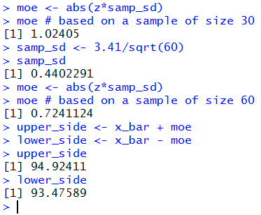
By increasing the sample size from 30 to 60
we changed the standard deviation of the sample means from
0.622578 (in Figure 3) to
0.4402291 (in Figure 4).
This changes the margin of error
from 1.02405 to 0.7241124.
Clearly, we can make the margin of error as small as we want
by increasing the sample size. But more on that later.
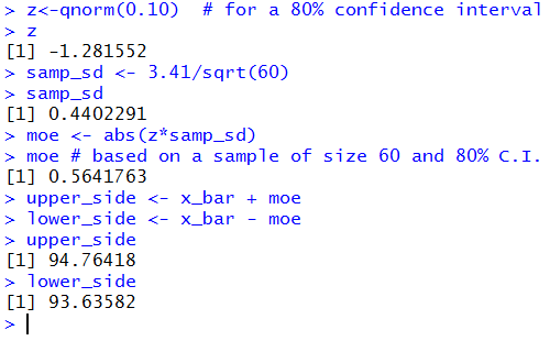
The other way that we can change the margin of error
is to change the desired confidence level. Figure 3
starts with us finding the required z-score so that we have 90%
of the area in the interval.
If we were to change that so that we only wanted
80% of the area in the interval then the value of |z| will be smaller,
that is, the z-score will be closer to 0.
This, in turn would make the margin of error smaller.
Figure 5 redoes the computations in our problem, still using
sample size 60, but now with a confidence level set
to 80%.
Figure 5
Clearly, reducing the sample size or raising the confidence level
will widen the confidence interval.
Look at some examples
In a previous web page we
were able to look at a population of 1000 values
where we set the population shape, mean, and standard deviation.
And we were able to draw 1000 random samples of some specified size and
see the sample mean (and sample standard deviation)
for each of those 1000 samples.
We will build on that by taking each of those sample means
and building a confidence interval from each one
with all the confidence intervals being built
with the same confidence level.
To do this we need to start at the
set up the arguments. page.
Figure 6 shows an image of that page with the
default values still in place.
Figure 6
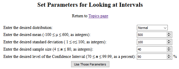
For our example we will just use those default values
and click on the "Use Those Parameters" button to
open a new page with our randomly generated population, our 1000 samples, and our 1000
confidence intervals, one from each sample mean.
As was true for the previous page,
all of this will be too long to display here, but I have saved a
pdf version of the page I generated
so that you can see the entire page if you want.
Also as before, we will "walk through" the page that was generated to point out the
various parts. Figures 7 through 13 cover the portion of the page that
has a structure identical to that
of the earlier page.
The new material dealing with confidence intervals starts in Figure 14.
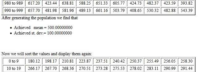
The page starts, as shown in Figure 7, with a confirmation
of the requested parameters followed by the first listing of the
population data.
Figure 7
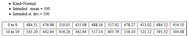
At the end of the listing the page displays the
mean and standard deviation for those
1000 values in the population.
After that is a sorted listing of the original values.
Figure 8
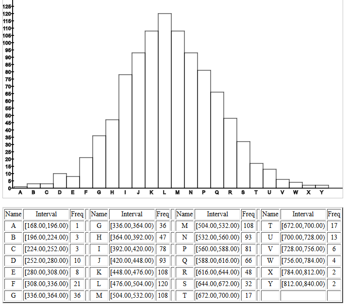
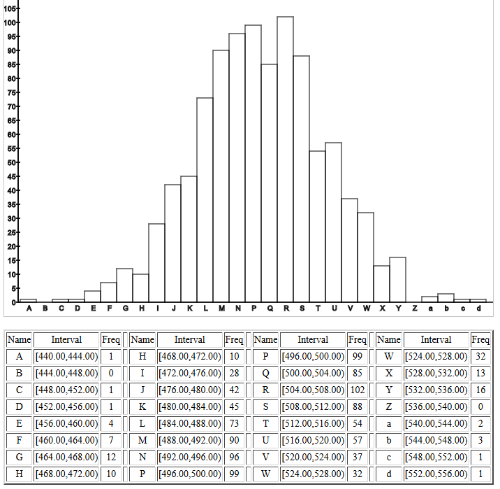
Following the sorted listing, the page holds a
histogram of the population values, followed by a table giving the
boundaries and actual frequencies for each of the
rectangles in the histogram. The histogram shown in Figure 9
fits the request for a normal distribution.
Figure 9
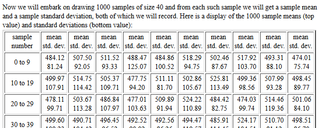
There is a "line printer" histogram (not shown here) before
the page gets to the start
of reporting the mean and standard deviation of the 1000 samples,
each of the requested size 40.
We are most interested in the sample means.
Figure 10 shows the first 40 such
sample means.
Figure 10
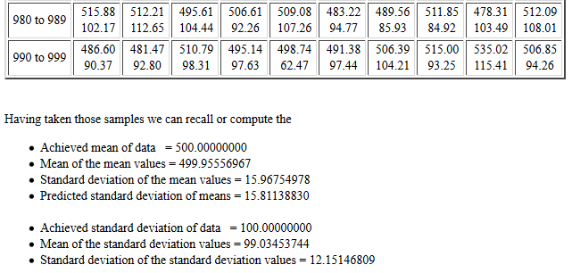
The listing of the sample statistic is followed by
the information shown in Figure 11.
In this case we see that the mean of the 1000
sample means is, as expected,
essentially the same as the population mean.
Furthermore, the
standard deviation of the sample means
is about 15.96755, a value quite close to the
value predicted by
 ,
15.81138830.
,
15.81138830.
Figure 11
This is followed by a histogram of the
sample means, reproduced in Figure 12.
Figure 12
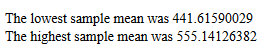
Following that histogram is a "line printer" version
(again not shown here) after which is a
quick report, Figure 13,
of the lowest and highest of the 1000
sample means. Up to this point, this
page has the identical structure
to that of the page that we used
to demonstrate taking samples.
Figure 13
Starting with Figure 14, this page takes the next steps.
|
Important Notice: This page was designed to show
more than the material presented thus far. In particular,
we are looking at the confidence intervals generated
when the standard deviation of the population is known.
Therefore, we will not be discussing the meaning of and the
results for confidence intervals when the
population standard deviation is unknown.
That will be done in
a subsequent page.
|
Figure 14 holds the introduction to the next part of the page.
Figure 14
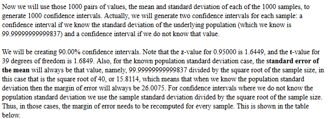
Part of that introduction is an explanation to show that
for all of the confidence intervals of interest here, the
margin of error will be the same, namely 26.0075.
Figure 15 shows the first few lines of the
table of confidence intervals,
one for each of the samples taken.
As noted above, here we are only concerned with the left
portion of the table, the highlighted portion in Figure 15.
Figure 15
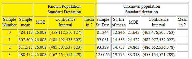
Examining Sample Number 0 in Figure 15 we see that
the mean of that sample was 484.119, the value
first reported back in Figure 10, though there it was given with only
2 decimal places. The margin of error is reported
as 26.008. Then the confidence interval
is (458.112,510.127). The next column
is left blank because the true population mean, 500, is in this
confidence interval.
Sample number 1 has a mean of 507.500 which
produces confidence interval of (481.492,533.507),
which also includes the population mean, 500.
Remember that the page generated 90% confidence intervals.
Therefore, about 90% of the intervals generated should
contain the mean of the population. All 4 of the samples
reported in Figure 15 generate confidence intervals
that contain the population mean.
Taking samples is a random event. As it turned out in this
case, the first time we get a sample that does not contain the true
mean is sample case number 40. That is not shown here, but you can see it in the
pdf file.
Instead, in Figure 16, we can see the second and third instances,
samples #65 and #69, where the generated confidence interval
does not contain the true mean. The fifth column in each of those is marked
FAIL. If you look at the pdf file and scan through all 1000
generated confidence intervals it is easy to pick out
the ones that have FAIL to indicate that they did not
contain the true population mean.
Figure 16
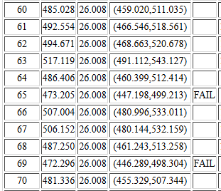
What happened in cases #65 and #69 is that the randomly selected
40 values that made up the sample produced a sample mean
that was so low that the generated confidence interval,
which has a margin of error = 26.008, does not contain
the value 500, the mean of the population.
There are other cases (#75, #106, #110, ...) where the sample mean is too high
and again the confidence interval misses the true mean.
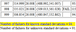
At the end of the table of confidence intervals
the web page ends with a count of the number of
intervals that failed to include the true mean.
This example page was constructed to get 90% confidence intervals.
Therefore, we expect that about 90% of the intervals generated will
contain the true mean.
That leaves 10% where the interval would
not contain the true mean. We took 1000 samples. 10% of 1000 is 100.
We expect about 100 of our intervals to miss the true mean.
Figure 17 reports that indeed 94 of our intervals missed the true mean.
Figure 17
It is worth the time and effort to go back and
use those web pages to generate numerous populations and samples
and confidence intervals, at different confidence levels,
and to see the
results which will be like those we have just seen in
our walk through in Figures 6 through 17.
Automating the process
The process of computing a confidence interval
in the case where we know the
population standard deviation and where
we have a sample of size n that yields a
sample mean is
as follows:
- From the confidence level compute the
value of using
- Use qnorm()
to find the associated z-score,
- Find the margin of error as
- Find the two parts to the confidence interval by evaluating
We should be able to describe these same actions using R
statements inside an R function.
Consider the following function definition:
ci_known <- function( sigma=1, n=30, x_bar=0, cl=0.95)
  {
    # try to avoid some common errors
    if( cl <=0 | cl>=1)
      {return("Confidence interval must be strictly between 0.0 and 1")
      }
    if( sigma < 0 )
      {return("Population standard deviation must be positive")}
    if( n <= 1 )
      {return("Sample size needs to be more than 1")}
    if( as.integer(n) != n )
      {return("Sample size must be a whole number")}
    # to get here we have some "reasonable" values
    samp_sd <- sigma/sqrt(n)
    z <- abs( qnorm( (1-cl)/2))
    moe <- z*samp_sd
    low_end <- x_bar - moe
    high_end <- x_bar + moe
    result <- c(low_end, high_end, moe, samp_sd)
    names(result)<-c("CI Low","CI High","MOE", "Std Error")
    return( result )
  }
This does all of our tasks, including returning the
confidence interval as well as some other values.
The function is available in the file
ci_known.R.
Figure 18 shows the console screen after the function has been entered
into an R session.
Figure 18
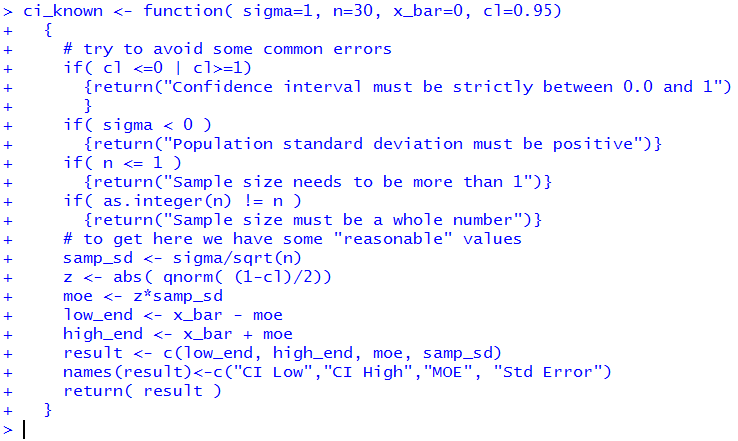
Figure 19 shows a use of the ci_known()
function to do the problem that
we did back in Figure 3. Fortunately, we get the same results.
Figure 19
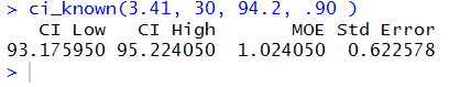
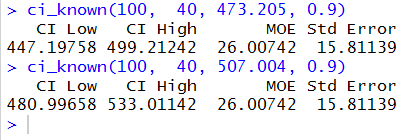
Figure 20 uses the information
needed to find the 90% confidence intervals
for samples #65 and #66 in Figure 16. Again,
the function produces the same values that had been on that
web page.
Figure 20
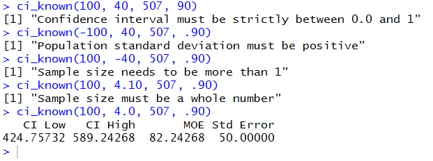
If you read the text of the function you know that it tries to trap any
obvious errors. Figure 21 shows a number of commands designed to
test out those traps. It is interesting to note that the final
example, specifying the sample size as 4.0, did not cause an error.
Apparently, R
has no problem if we use a decimal point in a whole number as long as
the value of the number is still an integer.
Figure 21
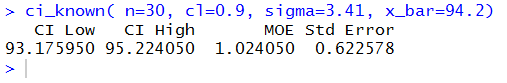
It can be difficult to remember the correct order of the
arguments in a call to the function. Figure 22 illustrates that we can name the
arguments, and, if we do so, we do not have to give them in order.
Again, this is the problem first done in Figure 3.
Figure 22
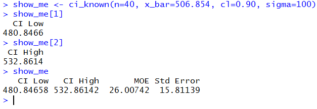
The working examples above show the function used by itself.
We could assign the results of the
function to a variable and then just examine parts or all of that variable.
This is done in Figure 23.
Figure 23
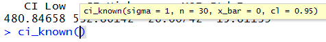
And, if we start typing the function
(after it has been defined, of course) into an R
session then R provides a little note to remind us of the needed
arguments. This also shows the default value of each argument.
It is true that if we wanted to take the default value then we need not specify it,
but that practice should be discouraged.
Figure 24
Interpreting A Confidence Interval
Let us say that we have a population
where we know the population standard deviation.
We choose a confidence level, perhaps 90%.
We take a sample and find the sample mean.
From all of that we can compute a 90% confidence interval.
It would be wrong to say "There is a 90% chance that the
true population mean is within the confidence interval."
The true population mean is either in the confidence interval or it is not!
It is not a question of probability! What we can and should say is "If I follow
the same procedure time and again, then 90% of the confidence intervals
that I generate will contain the true mean." That says nothing about the one
confidence interval that we did compute.
It says a lot about the method of computing it.
Visualizing Confidence Intervals
In the Fall 2025 semester some students requested a function to
help them "visualize" confidence intervals. The function
ci_known_visualize() attempts to do this.
For example, the sequence
source("../ci_known_visualize.R")
ci_known_visualize( 13.2, 38, 64.1 )
loads the function and then runs it for the case where the
population standard deviation is 13.2, the sample size is 38,
and the sample mean is 64.1. The output in the R-console is
> source("../ci_known_visualize.R")
> ci_known_visualize( 13.2, 38, 64.1 )
[1] "80 %  C.I. =( 61.356 , 66.844 )"
[1] "90 %  C.I. =( 60.578 , 67.622 )"
[1] "95 %  C.I. =( 59.903 , 68.297 )"
[1] "98 %  C.I. =( 59.119 , 69.081 )"
indicating confidence intervals for the 80%, 90%, 95%, and 98% levels.
In addition, the function produces the plot shown in Figure 25.
Figure 25
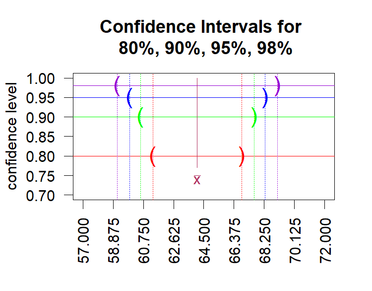
In that image you can see how the interval gets wider as we increase the
confidence level. Having a wider interval reflects the concept that more of such intervals
will contain the true mean.
Having created that function, and given the development of AI, one could
consider asking some AI to generate such a function. Here is a prompt given to
ChatGPT to do just that:
write an R function that will produce a plot to help the
user visualize confidence intervals for the mean when
the population standard deviation is known.
Arguments for the function should be the population
standard deviation, the sample size, and the sample mean.
The intervals produced should be at
the 80%, 90%, 95%, and 98% confidence level.
It is worth a try to see how ChatGPT, or a different AI machine,
responds to that prompt. Just a word of warning. Asking the same AI machine to do this
multiple times may well produce multiple, distinct solutions. Also, in some cases,
after trying the produced result, you may need to ask the AI machine to fix its solution
to either get it to run or to modify the output to your liking.
Worksheet for a Confidence Interval
Here is a link to a worksheet
with randomly generated problems related to
finding confidence intervals when the standard deviation of the population
is known.
Listing of all R commands used on this page
qnorm(0.025)
z<-qnorm(0.05)
z
x_bar <- 94.2
samp_sd <- 3.41/sqrt(30)
samp_sd
lower_side <- x_bar + z*samp_sd
lower_side
upper_side <- x_bar - z*samp_sd
upper_side

moe <- abs(z*samp_sd)
moe # based on a sample of size 30
samp_sd <- 3.41/sqrt(60)
samp_sd
moe <- abs(z*samp_sd)
moe # based on a sample of size 60
upper_side <- x_bar + moe
lower_side <- x_bar - moe
upper_side
lower_side

z<-qnorm(0.10)  # for a 80% confidence interval
z
samp_sd <- 3.41/sqrt(60)
samp_sd
moe <- abs(z*samp_sd)
moe # based on a sample of size 60 and 80% C.I.
upper_side <- x_bar + moe
lower_side <- x_bar - moe
upper_side
lower_side

ci_known <- function( sigma=1, n=30, x_bar=0, cl=0.95)
  {
    # try to avoid some common errors
    if( cl <=0 | cl>=1)
      {return("Confidence interval must be strictly between 0.0 and 1")
      }
    if( sigma < 0 )
      {return("Population standard deviation must be positive")}
    if( n <= 1 )
      {return("Sample size needs to be more than 1")}
    if( as.integer(n) != n )
      {return("Sample size must be a whole number")}
    # to get here we have some "reasonable" values
    samp_sd <- sigma/sqrt(n)
    z <- abs( qnorm( (1-cl)/2))
    moe <- z*samp_sd
    low_end <- x_bar - moe
    high_end <- x_bar + moe
    result <- c(low_end, high_end, moe, samp_sd)
    names(result)<-c("CI Low","CI High","MOE", "Std Error")
    return( result )
  }

ci_known(3.41, 30, 94.2, .90 )
ci_known(100,  40, 473.205, 0.9)
ci_known(100,  40, 507.004, 0.9)
ci_known(100, 40, 507, 90)
ci_known(-100, 40, 507, .90)
ci_known(100, -40, 507, .90)
ci_known(100, 4.10, 507, .90)
ci_known(100, 4.0, 507, .90)

ci_known( n=30, cl=0.9, sigma=3.41, x_bar=94.2)
show_me <- ci_known(n=40, x_bar=506.854, cl=0.90, sigma=100)
show_me[1]
show_me[2]
show_me

source("../ci_known_visualize.R")
ci_known_visualize( 13.2, 38, 64.1 )
Return to Topics page
©Roger M. Palay
Saline, MI 48176 December, 2015