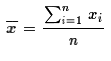
 , (and, although
we will not make much use of it, the sample standard deviation,
, (and, although
we will not make much use of it, the sample standard deviation,
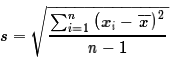 ).
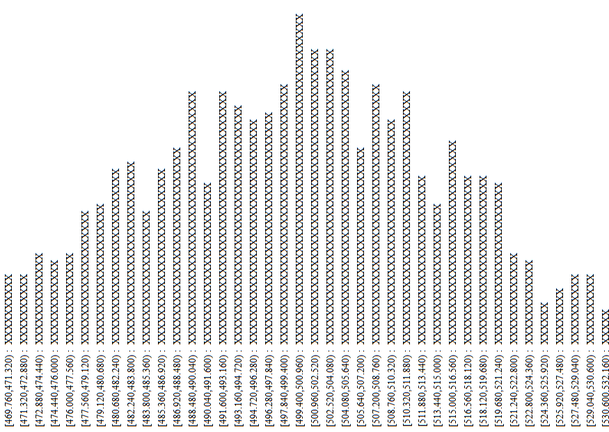
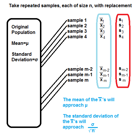
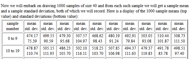
Then, we want to treat the collection of sample means
as a population itself and we want to examine the
mean and standard deviation of that population.
Figure 1 attempts to show this.
).
Then, we want to treat the collection of sample means
as a population itself and we want to examine the
mean and standard deviation of that population.
Figure 1 attempts to show this.
 .
.
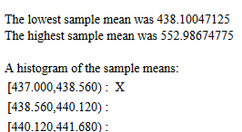
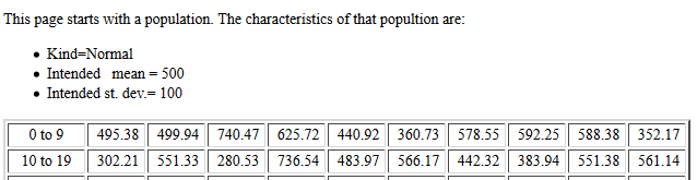
| It is important to note that each time you go to this subsequent page, or each time you refresh(reload) it, the new page will generate all new values for its population and it will take all new samples from that population. As such, the images shown below will have different values on them than the values you will see when you go to the page. |
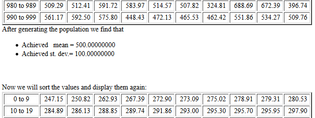

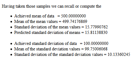 .
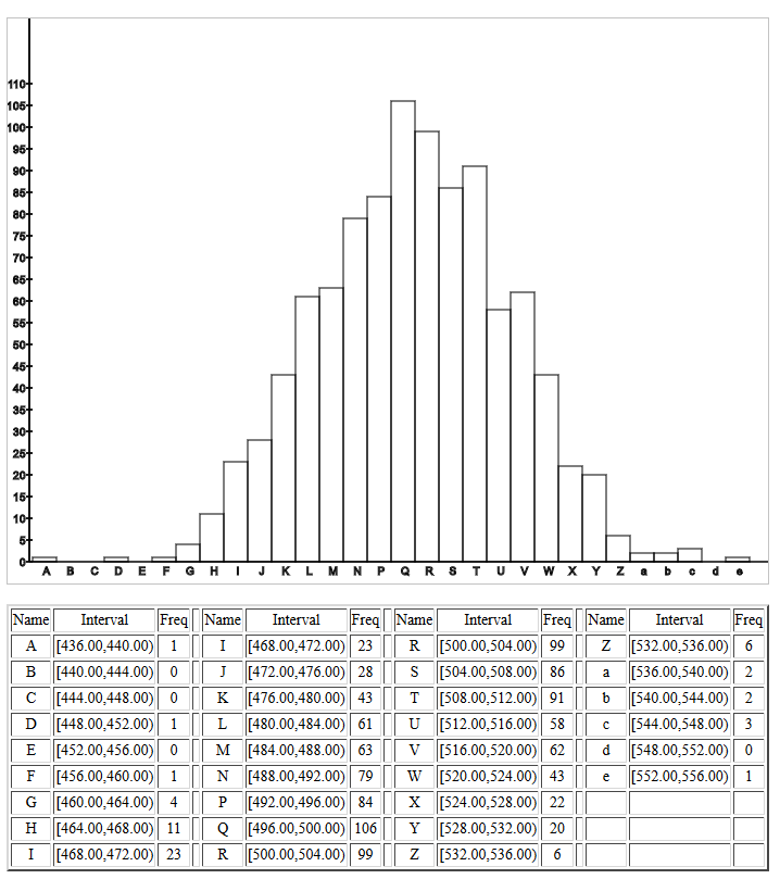
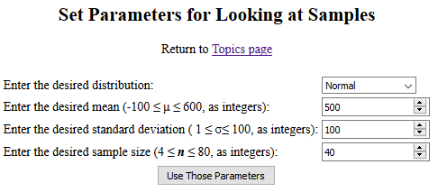
The population standard deviation was essentially 100.
The samples were of size 40.
The value of
.
The population standard deviation was essentially 100.
The samples were of size 40.
The value of  is about 15.8113883. This is the value expressed as the
"predicted value."
Thus, the actual standard deviation of the sample means
approaches .
is about 15.8113883. This is the value expressed as the
"predicted value."
Thus, the actual standard deviation of the sample means
approaches .