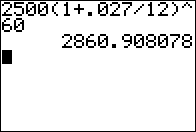
Figure 01
|
Find the future value when we invest $2500 at
2.7% the compounded monthly for 5 years (i.e., 60 months).
Use the formula
FVn = PV1(1 + r/t)n
Figure 01 shows evaluating the right side of the formula for those values
to get an answer of $2860.91.
|
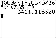
Figure 02
|
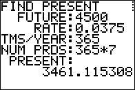
Find the present value
that will give us $4500 at the end of 7 years if we invest that
present value
at 3.75% compounded daily. [Note that for these kinds of calculations
it is common to use 365 as the number of days in a year.]
Use the formula
PV1 = FVn/(1 + r/t)n
Figure 02 shows evaluating the right side of the formula for those values
to get an answer of $3461.12.
|
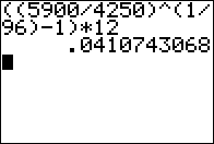
Figure 03
|
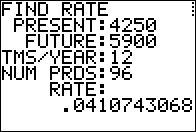
Find the rate that is required
to grow $4250 to a 5900 over 8 years compounded monthly.
Use the formula
r = ((FVn/PV1 )1/n - 1)*t
Figure 03 shows evaluating the right side of the formula for those values
to get an answer of 0.041074 or about 4.1%.
|
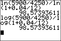
Figure 04
|
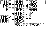
Find the
number of compounding periods required
to grow $4250 to $5900
when we know that we
will be compounding monthly at 4% annual interest.
Use either of the two versions of the formula,
one using the natural logarithm, ln() and the other using the
base-10 logarithm, log()
n = ln(FVn/PV1) / ln(1 + r/t) = log(FVn/PV1) / log(1 + r/t)
Figure 03 shows evaluating the two versions of the formula for those values
to get an answer of 98.5739, which means 8 years and just over 2 and a jhalf months.
|
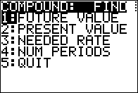
Figure 05
|
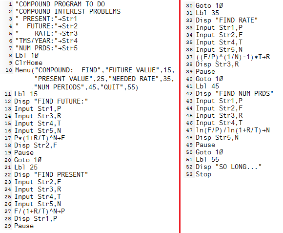
Once the program starts we see the menu created by line 10 in the program.
|
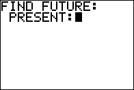
Figure 06
|
Choosing the first option takes us to line 11 and from there to
line 12 to display "FIND FUTURE", and then
the calculator prompts us with the contents of Str1, leaving us at Figure 02.
|
Figure 07
|
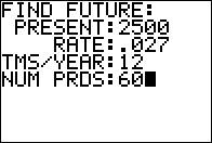
Responding to the prompt with 2500 and then the
 key, the program stores the 2500 in the
variable P and then goes on to ask for the rate. In Figure 07
we see the status of the program after we have given it all the requested information.
Press key, the program stores the 2500 in the
variable P and then goes on to ask for the rate. In Figure 07
we see the status of the program after we have given it all the requested information.
Press  to have the calculator
accept the last value and move on to display the answer. to have the calculator
accept the last value and move on to display the answer.
|
Figure 08
|
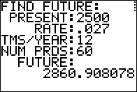
Figure 08 shows that answer. After verifying that this is the same result
that we had in Figure 1, we press  and
the calculator returns to the menu, shown in Figure 09. and
the calculator returns to the menu, shown in Figure 09.
|
Figure 09
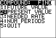
|
Now we can select the second option.
|
Figure 10
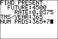
|
That brings us to Figure 10 where we have entered all
the values in the second problem from Figure 02.
Again, press  to continue. to continue.
|
Figure 11

|
The answer shown in Figure 11 is the same as the one we found in
Figure 02.
|
Figure 12

|
Without showing the return to the menu and then moving forward,
Figure 12 shows the values and answer for the third type of problem.
|
Figure 13

|
Figure 13 shows the values and the answer for the fourth kind
of problem.
|
Figure 14

|
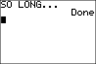
And, Figure 14 shows the result of selecting the QUIT option
in the menu.
|




 key, the program stores the 2500 in the
variable P and then goes on to ask for the rate. In Figure 07
we see the status of the program after we have given it all the requested information.
Press
  to have the calculator
accept the last value and move on to display the answer.

 and
the calculator returns to the menu, shown in Figure 09.


 to continue.
