


|
First we will observe a fact or two. Press then 
  to get Figure 1. Note the up-arrow
in the cursor block indicating that we are in the yellow shift mode. to get Figure 1. Note the up-arrow
in the cursor block indicating that we are in the yellow shift mode.
|
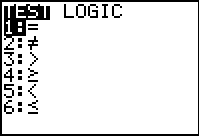 |
Now, press the  key to open the TEST menu shown in Figure 2.
We want to choose the "greater than" sign, which is option 3. We do this by pressing
the key to open the TEST menu shown in Figure 2.
We want to choose the "greater than" sign, which is option 3. We do this by pressing
the  key. This will paste teh "greater than" sign into our expression. key. This will paste teh "greater than" sign into our expression.
|
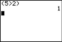 |
Here we see that the "greater than" sign is in our expression. We complete that expression
with the   sequence and
then use the sequence and
then use the  to evaluate the expression. The
calculator responds with the value 1. This demonstrates that the value of "TRUE"
is evaluated as 1. to evaluate the expression. The
calculator responds with the value 1. This demonstrates that the value of "TRUE"
is evaluated as 1.
|
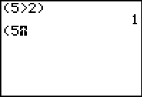 |
We start the next expression with the same 
  keys. keys.
|
 |
Press the  key to return to the TEST menu.
This time we will select option 6, less than or equal. We do this
by pressing the key to return to the TEST menu.
This time we will select option 6, less than or equal. We do this
by pressing the  key. key.
|
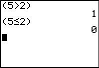 |
Again, the symbol has been pasted into the expression. We complete the expression
with   and
press and
press  to evaluate the expression.
The calculator responds with 0. Thus, the value FALSE is evaluated to 0. to evaluate the expression.
The calculator responds with 0. Thus, the value FALSE is evaluated to 0.
|
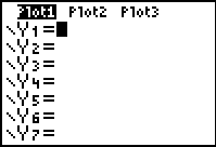 |
The  key opens the Y= screen shown in Figure 7.
We will use the fact that TRUE is 1 and FALSE is 0 along with the the
facts that 1 times a value is that same value,
0 times a value is 0, and 0 plus a value is that same value to
help enter our piecewise function. key opens the Y= screen shown in Figure 7.
We will use the fact that TRUE is 1 and FALSE is 0 along with the the
facts that 1 times a value is that same value,
0 times a value is 0, and 0 plus a value is that same value to
help enter our piecewise function.
|
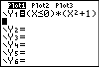 |
We start with the expression (x 0)*(x2 + 1).
Whenever x is less than or equal to 0, the first factor,
(x 0)*(x2 + 1).
Whenever x is less than or equal to 0, the first factor,
(x 0), will have the value 1 so the entire expression
will just have the value (x2 + 1). On the other hand, if x is greater than
0, the first factor will have the value 0 so the whole expression will have the
value 0 and it will not change the value of anything that we add to it. 0), will have the value 1 so the entire expression
will just have the value (x2 + 1). On the other hand, if x is greater than
0, the first factor will have the value 0 so the whole expression will have the
value 0 and it will not change the value of anything that we add to it.
|
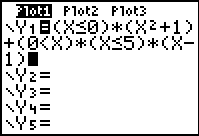 |
In Figure 9 we continue the definition of the piecewise function by adding the second portion as
(0 x)*(x x)*(x 5)*(x-1). If x
less than or equal to 0 then the first factor is 0 so the entire expression will be 0.
If x is greater than 5 then the second factor is 0 so the entire expression will be 0.
It is only in the case that x is greater than 0 and x is
less than or equal to 5 that both first factors will have the value 1, in which case the
third factor (x-1) determines the value of this expression. 5)*(x-1). If x
less than or equal to 0 then the first factor is 0 so the entire expression will be 0.
If x is greater than 5 then the second factor is 0 so the entire expression will be 0.
It is only in the case that x is greater than 0 and x is
less than or equal to 5 that both first factors will have the value 1, in which case the
third factor (x-1) determines the value of this expression.
|
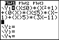 |
We complete the piecewise function in Figure 10 with the last term,
(x 5)*(3x-11). This term will be 0 for
all values of x less than or equal to 5. For values of x greater than 5
the factor (x 5)*(3x-11). This term will be 0 for
all values of x less than or equal to 5. For values of x greater than 5
the factor (x 5) evaluates to 1 making the value of this third term be
defined by the value of the second factor, (3x-11). 5) evaluates to 1 making the value of this third term be
defined by the value of the second factor, (3x-11).
|
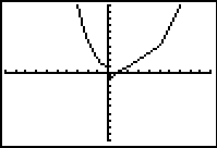 |
pressing the  produces the graph of the piecewise function shown in Figure 11.
|
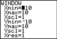 |
To complete this examination, we want to look more closely at the function
for values of x between -2 and 8. We open the
WINDOW screen, shown in Figure 12 by presing the  key. key.
|
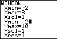 |
Figure 13 shows the changes we have made. |
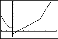 |
Pressing  produces the graph in Figure 14. This looks OK, until you really look at it.
There is a small problem near the origin. Here is a magnified version of that area, but with the
questionable pixels in red: produces the graph in Figure 14. This looks OK, until you really look at it.
There is a small problem near the origin. Here is a magnified version of that area, but with the
questionable pixels in red:  We cannot explain those pixels by looking at the piecewise function definition. |
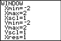 |
In an attempt to look at this more closely, we return to the WINDOW screen,
via the  key, and we make the changes shown in Figure 15.
Then, press the key, and we make the changes shown in Figure 15.
Then, press the  key to move to Figure 16. key to move to Figure 16.
|
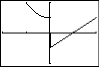 |
This is more perplexing because there are now extra pixels to the right and below the origin,
highlighted in red in the
following:  and the offending pixels from Figure 14 have disappeared. |
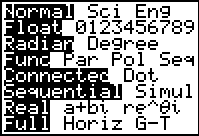 |
The cause of all of this can be traced back to our original MODE settings.
Figure 17 has the MODE
screen as the result of pressing the  key.
The fifth option from the top is the choice between Connected and Dot.
In connected mode, the current setting, the TI-83 as it graphs
points of the function, tries to connect those points by
filling in the vertical pixels between the points.
A more lengthy discussion of this is in the pixels web page.
We can just illustrate the featue here by changing this setting and then returning to the graph. key.
The fifth option from the top is the choice between Connected and Dot.
In connected mode, the current setting, the TI-83 as it graphs
points of the function, tries to connect those points by
filling in the vertical pixels between the points.
A more lengthy discussion of this is in the pixels web page.
We can just illustrate the featue here by changing this setting and then returning to the graph.
|
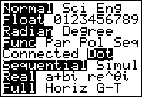 |
For Figure 18 we have moved the highlight over the Dot option and then
pressed the  key. key.
|
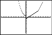 |
Press the  key to open the ZOOM window,
the key to open the ZOOM window,
the  key to select the standard view, i.e., WINDOW settings, and key to select the standard view, i.e., WINDOW settings, and
 key to reurn to the graph.
The offending dots have gone away, but so has the connected nature of the graph. key to reurn to the graph.
The offending dots have gone away, but so has the connected nature of the graph.
|
©Roger M. Palay
Saline, MI 48176
August, 2010