Figure 1

|
We start this sequence on the Y= screen by pressing the
 key.
We note in Figure 1 that the calculator used here has a function defined for Y1.
For the purpose of this page we do not want that function defined at this time.
Therefore, we will clear the function by pressing the key.
We note in Figure 1 that the calculator used here has a function defined for Y1.
For the purpose of this page we do not want that function defined at this time.
Therefore, we will clear the function by pressing the  key. This will produce Figure 2.
|
Figure 2

| Figure 2 has no functions defined for graphing.
If need be, we could have cleared other functions by moving the cursor to
those functions and pressing the CLEAR key. The important point here is that we have
cleared all graphing functions.
|
Figure 3

| We move to Figure 3 by pressing the  key. That will bring up the ZOOM menu shown here. We can select any of the
options, but the one that we will use is option 4: ZDecimal
We select that option by pressing the
  key.
This will set certain default values for the minimum and maximum values
that can be displayed on the screen, and it will move us to the graph screen
shown in Figure 4. key.
This will set certain default values for the minimum and maximum values
that can be displayed on the screen, and it will move us to the graph screen
shown in Figure 4. |
Figure 4

| The calculator used here did not have any plots of points defined, and
it did not have any graphing functions defined (we cleared those in Figures 1 and 2).
Therefore, the graph has nothing on it but the axes. We can tell a good deal
from the graph of the axes. Figure 4A is a reproduction of Figure 4, but with
certain features identified.
|
Figure 4A
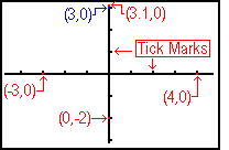
| The ZDecimal option that we used to generate Figure 4 sets the parameters for the
screen so that the middle of each pixel has coordinates that are exact decimal values to
one decimal place to the right of the decimal point. That is, these points all
have coordinates that are in even tenths.
In Figure 4A we have identified the "tick marks" that help us divide up the X
and Y scales. In addition, we have identified the particular pixels that
represent certain ordered pairs.
We can see the actual settings for the minimum and maximum values, and the frequency for
the "tick marks" by moving to the WINDOW screen. We do
this by pressing the  key. This will move us to Figure 5. key. This will move us to Figure 5.
|
Figure 5

| Figure 5 was captured from the calculator screen as the blinking cursor
covered the minus sign before the Xmin value of -4.7. In Figure 5 we can see the
values that have been assigned to Xmin, Xmax, Ymin, and Ymax.
If we remember that there are 95 columns of pixels, then we can see that we
can assign the Xmin value, -4.7, to the leftmost column,
-4.6 to the next column to the right, -4.5 to the next column,
and so on. Eventually, we will assign the middle column to 0 and then the next column
to 0.1, and so on until we get to the 95th column, which we will assign to 4.7,
which is the Xmax value.
Similarly, there are 63 rows of pixels. We can assign the bottom row to -3.1, the row above it
to -3.0, and so on, including the middle row being
assigned to 0 and the 63rd row being assigned
to 3.1. Note that there is another value on the screen, namely Xres.
We will discuss that value in Figure 23.
|
The text above was careful to imply that values are associated with pixels. Once the
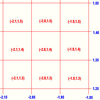 Xmin, Xmax, Ymin, and Ymax values have been set,
we can determine the boundaries for each pixel.
The figure at the right is meant to represent a small portion, 9 pixels, from
the graph above. Each pixel has a small dot in its center and the coordinates of
that dot are given inside each cell. We note that there is much more to each pixel than the labeled
point in the center. On the outside of the figure we have the values that must be
at the boundary of each pixel. Thus, the very center pixel, the one with the point
(-2.0,1.4) must represent all of the X-values between -2.05 and -1.95 paired with
Y-values between 1.35 and 1.45. If the calculator is trying to graph
or plot a point that falls into the ranges just given, then it is the center pixel
in the figure that will get turned black. Thus, each of the points
Note that there is a small problem here. The point
We will use the TI-83 to generate a plot of six different points in order to illustrate some of this.
Figure 6

| To generate a plot we need to enter some values into lists.
The TI-83 has six standard lists. We will use L1 and
L2. To do this, we want to make sure that those lists are
in the list editor. We can do this first step from the STAT
menu. We press the  key to open the STAT menu as seen in
Figure 6. key to open the STAT menu as seen in
Figure 6. From this menu, we need to choose option 5: SetUpEditor.
We do this by pressing the  key to paste
SetUpEditor onto the main screen. key to paste
SetUpEditor onto the main screen. |
Figure 7

| Figure 7 shows the main screen after we have pasted
SetUpEditor and after we have pressed the
 key to have the calculator perform that command.
The only confirmation that we get is the word Done on the right of the screen. key to have the calculator perform that command.
The only confirmation that we get is the word Done on the right of the screen. |
Figure 8

| The next step is just a convenience for us. We will clear all of the
lists on the calculator. This will save us from having to worry about
values that were previously stored. We will clear all of the lists by using the command
ClrAllLists on the MEM menu. To do this we press
  to open the menu, shown in Figure 8. The option we want is #4.
We press the
  to select this option. to select this option. |
Figure 9

| Figure 9 shows the result of making our selection and
of pressing the  key to perform the command.
Again, the calculator responds with the word Done. key to perform the command.
Again, the calculator responds with the word Done. |
Figure 10

| We return to the STAT menu, via the  key, so that we can start to edit the lists L1 and
L2. We press the
  key to select the highlighted option, 1:Edit. This will move us to Figure 11.
|
Figure 11

| We are ready to start entering values into the lists. The highlight is on the
spot where we can enter the first value for
L1. The points that we want to enter are:
(-4.66,2.9)
(-4.64,2.5)
(-4.56,2.0)
(-4.54,1.5)
(-4.7,1.0)
(-4.71,0.5)
The X-coordinates need to be placed into the L1 list,
and the Y-coordinates need to be placed into the L2 list.
|
Figure 12

| We start by entering the -4.66, pressing the keys,
  
  and then and then  .
The result is shown in Figure 12. Note that we are ready for the next X-coordinate. .
The result is shown in Figure 12. Note that we are ready for the next X-coordinate.
|
Figure 13

| Figure 13 shows the list after we have entered each of the six X-coordinates.
The calculator is ready to receive a seventh, but we are done withour values. Therefore,
we press the  key to move to the
L2 list. key to move to the
L2 list.
|
Figure 14

| We have moved to the L2 list and the calculator is ready to
accept the Y-coordinates. |
Figure 15

| In Figure 15 we have completed entering all of the coordinates. We are
done with the data entry process.
We can QUIT this by pressing   .
This returns us to the main screen, shown in Figure 16, just as we left it in Figure 9. .
This returns us to the main screen, shown in Figure 16, just as we left it in Figure 9. |
Figure 16

| At this point we have entered the values in the two lists,
but we have not told the calculator that we want it to plot those values.
We can start this process by moving to the STAT PLOT screen. |
Figure 17

| We get to the STAT PLOT screen by pressing
  .
Figure 17 shows the result. This screen shows four options. The first
option, if selected, will allow us to change the settings associated with
Plot1. As a convenience to us, the calculator shows, on the
STAT PLOT screen, the settings that are in effect for PLOT1.
First, Plot1 is set "Off". This means that it will not be plotted.
Second, the plot is to be a scatter plot. Third,
Plot1 is going to use L1 and L2 .
And, fourth, Plot1 will use the square symbol, .
Figure 17 shows the result. This screen shows four options. The first
option, if selected, will allow us to change the settings associated with
Plot1. As a convenience to us, the calculator shows, on the
STAT PLOT screen, the settings that are in effect for PLOT1.
First, Plot1 is set "Off". This means that it will not be plotted.
Second, the plot is to be a scatter plot. Third,
Plot1 is going to use L1 and L2 .
And, fourth, Plot1 will use the square symbol,  ,
to mark each of the points to be plotted.
The one setting that we need to change is the first, from Off to On.
The STAT PLOT screen does not allow us to make this change. Instead, we need to select
option 1 to move us to a new screen, dedicated to the Plot1 settings.
We can select option 1 by pressing the ,
to mark each of the points to be plotted.
The one setting that we need to change is the first, from Off to On.
The STAT PLOT screen does not allow us to make this change. Instead, we need to select
option 1 to move us to a new screen, dedicated to the Plot1 settings.
We can select option 1 by pressing the  key. key.
|
Figure 18

| Figure 18 shows the screen that allows us to change the settings for Plot1.
When Figure 18 was captured from a calculator, the blinking cursor was covering the "On" option.
The "Off" value is highlighted because it is the current setting.
Since the cursor is at the "On" option, we can change that setting by pressing the
 key.
THis will change the display to that of Figure 19. key.
THis will change the display to that of Figure 19.
|
Figure 19

| Note in Figure 19 that the blinking cursor is still at the "On" value, but
the "On" value is also highlighted. We have turned "On" Plot1.
We can see the effect of this change
by pressing the  key to display the graph. key to display the graph. |
Figure 20

| Here we have the plot of the points in
L1 and L2. We need to examine this plot
with respect to the values that we know are being plotted and remembering the WINDOW settings
that are in effect. First, note that although we defined six points in
L1 and L2, there are only
five points that are plotted.
The last point, (-4.71,0.5), has not been plotted. If we recall the true limits
to each pixel, we can calculate that the leftmost column of pixels are associated with
the numbers -4.75 through -4.65. Our sixth point, (-4.71,0.5), falls within this range.
However, for the pixels at the edge of the screen, the
calculator uses the Xmin, Xmax, Ymin, and Ymax values
as the limit to what it will plot, even if the desired
value is just slightly outside of the given range.
|
Figure 20A (Augmented)

| Figure 20 has been repeated in an augmented form in Figure 20A.
Here we have given the coordinates of the five points that were plotted.
We note that the topmost point has coordinates (-4.66,2.9)
and that point should be in the leftmost column of the screen, the one
associated with the range of X-values -4.75 through -4.65. Even though we are just
into that range, it is indeed the leftmost column that is identified, by having the
small square,  ,
placed around it. Indeed, because this is the leftmost column, the
left third of the square can not be shown. ,
placed around it. Indeed, because this is the leftmost column, the
left third of the square can not be shown.
The next two points have coordinates (-4.64,2.5) and (-4.56,2).
Both fall into the range of values associated with the second column of pixels, namely,
values from -4.65 through -4.55. Therefore, the pixels that are associated with these points are
both in that same second column of pixels.
|
Figure 20A (Repeated)

| Again, in Figure 20A, the fourth point has coordinates
(-4.54,1.5).
The X-coordinate, -4.54, is just less than the right boundary value for the second column
of pixels, -4.55. Therefore, the fourth point is plotted in the next, the third, column of
pixels.
The last point to be plotted has the X-coordinate -4.7. This is the value of Xmin.
It is the lowest X-value that can be plotted on this graph.
|
Figure 21

| Until now we have plotted points. But what if we want to graph a function
such as Y=4X+1?
First we need to enter the function. We press  to move to the Y= screen shown in Figure 21.
|
Figure 22

| In Figure 22 we have defined the function by pressing the keys
  
 |
Figure 23

| We return to the GRAPH screen by pressing
 . Note that we did not turn off the plot, so our points
are still plotted. However, in Figure 23 we also have the graph of the function.
A close examination of the graph of the function shows that it is made up of
a number of small vertical segments. Why? . Note that we did not turn off the plot, so our points
are still plotted. However, in Figure 23 we also have the graph of the function.
A close examination of the graph of the function shows that it is made up of
a number of small vertical segments. Why?
To generate the graph, the TI-83 tries different
values of X and it generates the corresponding values for Y. What values
does it use? It starts at the minimum X-value, Xmin, and it tries that value.
Then it finds the next value by moving to the center X-value in a pixel Xres
steps to the right.
Xres was defined in the WINDOW settings that we saw back in Figure 5.
Thus, we start X at the minimum value, -4.7, and get a value for Y.
If that point can be plotted, then the calculator graphs it. It then moves Xres pixels to the right.
Since Xres is 1 for this graph,
the calcualtor selects the center value in the second column, namely -4.6.
Again, the calculator uses that X-value to determine a Y-value, and the resulting point is
plotted if it is on the screen. This process is repeated until we have moved across all 95 columns
of pixels.
Thus, for the function Y=4X+1,
the X-value 0.3 should produce the Y-value 2.2,
0.4 should produce 2.6, and 0.5 should produce 3.0.
These points, (0.3,2.2), (0.4,2.6), and (0.5,3.0),
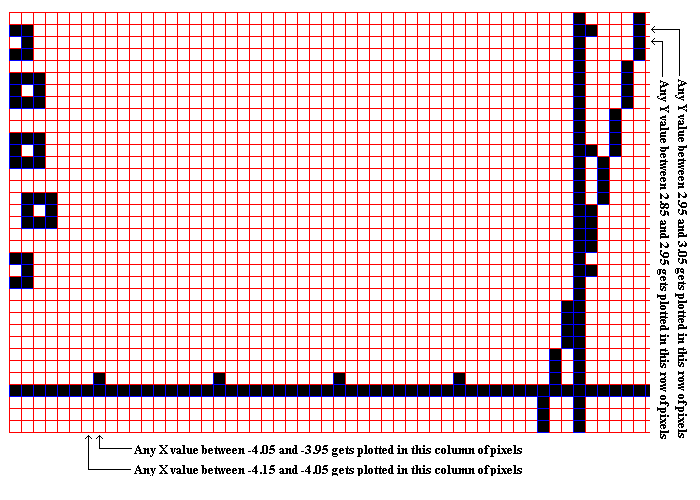
would be graphed in adjacent columns of pixels, but not adjacent rows. You can identify
each of the pixels in the following, magnified and enhanced image of a portion of Figure 23.
|
Here is a reproduction of Figure 27, but magnified.

 key.
We note in Figure 1 that the calculator used here has a function defined for Y1.
For the purpose of this page we do not want that function defined at this time.
Therefore, we will clear the function by pressing the
  key. This will produce Figure 2.


 key. That will bring up the ZOOM menu shown here. We can select any of the
options, but the one that we will use is option 4: ZDecimal
We select that option by pressing the
  key.
This will set certain default values for the minimum and maximum values
that can be displayed on the screen, and it will move us to the graph screen
shown in Figure 4.

 key. This will move us to Figure 5.

 Xmin, Xmax, Ymin, and Ymax values have been set,
we can determine the boundaries for each pixel.
The figure at the right is meant to represent a small portion, 9 pixels, from
the graph above. Each pixel has a small dot in its center and the coordinates of
that dot are given inside each cell. We note that there is much more to each pixel than the labeled
point in the center. On the outside of the figure we have the values that must be
at the boundary of each pixel. Thus, the very center pixel, the one with the point
(-2.0,1.4) must represent all of the X-values between -2.05 and -1.95 paired with
Y-values between 1.35 and 1.45. If the calculator is trying to graph
or plot a point that falls into the ranges just given, then it is the center pixel
in the figure that will get turned black. Thus, each of the points

 key to open the STAT menu as seen in
Figure 6.
 key to paste
SetUpEditor onto the main screen.
 key to have the calculator perform that command.
The only confirmation that we get is the word Done on the right of the screen.

 to open the menu, shown in Figure 8. The option we want is #4.
We press the


 key to move to the
L2 list.


 .
This returns us to the main screen, shown in Figure 16, just as we left it in Figure 9.
 key.
key.


 key to display the graph.




 key four times to move the cursor
to that row of options, and then pressing the

