We need to start with some data.
We will generate a list of data on the calculator using
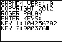
GNRND4 with Key 1=104256702 and Key 2=900376. That list
will be the same numbers that appear in the following table:
Thus, our problem will be to generate a Pareto chart for the data in the
list above. A Pareto Chart is just a bar chart but with the
items arranged in decreasing order of frequency. Therefore, our first steps will
be exactly the same as the steps we would take to do a bar chart.
Figure 1
|
We start the GNRND4 program and give it the two key values.
|
Figure 2
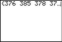 |
After a few screens, the program displays the
contents of L1.
We note that these are exactly the values in the table above.
The program is still running at this point, so we
can press  to have it continue to the end. to have it continue to the end.
|
Figure 3
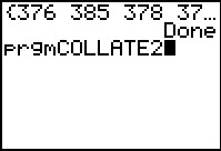 |
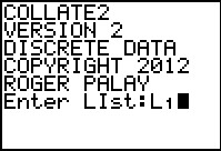
GNRND4 has completed. Although we need not do it now, we will
run the COLLATE2 program at this point. After that,
starting in Figure 7, will have the calculator do a bar graph of the data.
It is important to note that the
calculator will do that bar graph on the data in
L1. It does not need or use the output
of COLLATE2. We run COLLATE2 here just to give us some information.
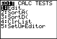
In Figure 3 we have already selected COLLATE2 from the list of programs on the calcualtor.
We will press to start the program.
|
Figure 4
 |
The program displays some information and then it asks for the data list.
We respond with L1.
Again, we will press to have the
program accept our response and continue running.
|
Figure 5
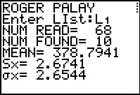 |
The program produces some display output. Here we note that
the program found 10 different values among the 68 items in the list.
The program is in a "paused" state. We press
to have it continue.
|
Figure 6
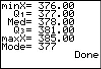 |
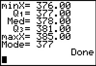
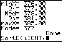
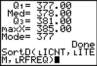
The rest of the display output is shown in Figure 6. In particular,
we note that the values in the original list range from 376 to 385.
COLLATE2 does more than jsut produce the display information. It also created some new lists.
We will return to see these in Figure 15.
|
Figure 7
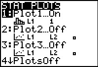 |
Once COLLATE2 has completed, we press 
 so that we can be sure that Plot1 is "On" (it is) ,
that it is set to do a "histogram" (it is), and that it will do that histogram
on the data in L1 (it is).
If these values were not set correctly then we would have had to open the Plot1
menu and correct them. so that we can be sure that Plot1 is "On" (it is) ,
that it is set to do a "histogram" (it is), and that it will do that histogram
on the data in L1 (it is).
If these values were not set correctly then we would have had to open the Plot1
menu and correct them.
|
Figure 8
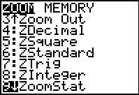 |
Pressing  takes us to the
ZOOM menu. There we use the takes us to the
ZOOM menu. There we use the  key to move down the list to find our
desired option ZoomStat. Once we have found and highlighted that option
we press to select it. This will cause the
calculator to examine the data in L1 and tehn to set the
WINDOW values appropriately for a histogram. It also causes that historgram to be displayed,
as in Figure 9.
key to move down the list to find our
desired option ZoomStat. Once we have found and highlighted that option
we press to select it. This will cause the
calculator to examine the data in L1 and tehn to set the
WINDOW values appropriately for a histogram. It also causes that historgram to be displayed,
as in Figure 9.
|
Figure 9
 |
lthough this is a valid histogram, it is notthe bar chart that we want.
There are only 8 bars to cover the 10 values that we know are in the list of the original data.
|
Figure 10
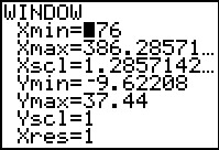 |
We press the  key to move to the WINDOW
menu. Here we see the values that the calculator determined to be appropriate.
We want to change some of those values. key to move to the WINDOW
menu. Here we see the values that the calculator determined to be appropriate.
We want to change some of those values.
|
Figure 11
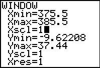 |
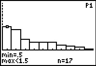
The new values typed into the menu shown in Figure 11 have the low end of the first class
startign at 375.5 with a class width of 1 and the low end of the class following or final display class
starting at 385.5.
|
Figure 12
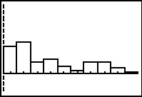 |
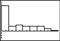
We press the  key to get the new graph shown in Figure 12.
This is almost what we want, but this is a bar chart, not a Pareto chart.
The difference is that the Pareto chart needs to have the items
arranged in decreasing order of frequency. At this point we cannot do this on the calculator.
However, there may be sonme things that we can do. key to get the new graph shown in Figure 12.
This is almost what we want, but this is a bar chart, not a Pareto chart.
The difference is that the Pareto chart needs to have the items
arranged in decreasing order of frequency. At this point we cannot do this on the calculator.
However, there may be sonme things that we can do.
|
Figure 13
 |
We exit the graph display by
pressing  .
This returns us to our main screen. .
This returns us to our main screen.
|
Figure 14
 |
Press  to open the STAT menu.
Press to select the Edit option. to open the STAT menu.
Press to select the Edit option.
|
Figure 15
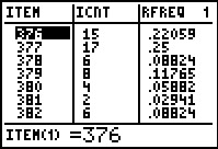 |
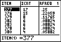
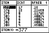
Figure 15 is from the Stat Editor. Here we see the more hidden results
of running COLLATE2 before, namely, we have some special lists
and they are displayed in the editor.
|
Figure 16
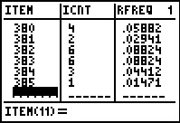 |
We use the key to scroll down to see the rest of the values.
We could stop our calculator work here. After all, we have 10 rows of values
and we could sort those rows by hand putting the row with 17 in
LICNT at the top,
followed by the row with 15 in LICNT,
followed by the row with 8 in LICNT, and so on.
Then we can construct, by hand, a Pareto chart by using the associated
frequencies to determine the height of each bar on the chart. If we make the first bar,
the one associated with the value 377, 10 centimeters tall, then the
height of the bar representing 376, with 15 as its frequency will
be determined by 15*(10/17). This calculation was
presented and discussed in the material on bar charts.
On the other hand, perhaps we can get the
calculator to sort this information for us.
|
Figure 17
 |
As usual, we exit the editor via the sequence
|
Figure 18
 |
At a minimum, we want to sort the LICNT
list into descending order. However, we want to do this while we keep the information in
at least the LITEM list, and most likely the
LRFREQ list, associated with the same value
in LICNT. That is, at the start we have the
second entry in each of the three lists related: (as we see in Figure 15) 377 is related to
17 and that is related to .25. It would not do us much good to
just sort LICNT without moving the values in the other lists
to keep things line up.
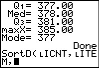
Fortunately, the SortD( command will do this for us.
We want to construct the command
SortD(LICNT,
LITEM,
LRFREQ)
This will sort the first list into descending order while moving the items in the other lists in parallel
with the items in the first list.
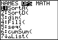
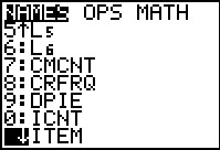
We start building our command by moving to the LIST menu via
, and then moving tot he
OPS sub-menu by using the  key. Then we can choose
SortD(, the second option, by pressing the key. Then we can choose
SortD(, the second option, by pressing the  key. key.
|
Figure 19
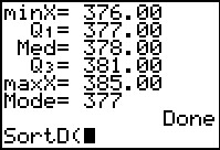 |
Figure 19 shows that we ahve pasted
the SortD( command onto the main screen.
|
Figure 20
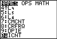 |
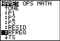
We move back to the LIST menu,
,
and then move down to
find our desired entry, LICNT.
Press to select that name.
|
Figure 21
 |
The name has been pasted and
we have followed that by the  . .
|
Figure 22
 |
It is back to the LIST menu, find the next name that we want,
and then select that name.
|
Figure 23
 |
The name has been pasted and we follow it with another
.
|
Figure 24
 |
Return to the LIST menu, find the last name, select it.
|
Figure 25
 |
We complete the command with the  .
Once the command is complete we press
to have the calcualtor perform it. .
Once the command is complete we press
to have the calcualtor perform it.
|
Figure 26
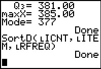 |
The calculator responds with Done to indicate that the processing has completed.
We move back via STAT, Edit to see the editor in Figure 27.
|
Figure 27
 |
In this figure we see that the values have been sorted, and that the associated values
in the other two columns have moved with the value in
LICNT.
|
Figure 28
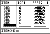 |
Figure 28 shows the bottom of the lists.
|
Figure 29
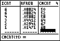 |
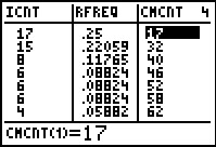
Before we leave this, we have moved over to see one of the other columns
namely LCMCNT
This was not sorted with the other columns. Therefore,
the values in this list no longer correspond to the
values in the sorted columns. A quick look shows that 50 in
LCMCNT is associated with the top 6
in LICNT.
However, the next line in LICNT is another 6.
That means that we should have 6 added to the cumulative total which is in
LCMCNT, but we find 52 there instead.
|
It would seem that we are stuck at this point. The calculator will do a
bar chart of the data and that bar chart has
all of the required columns but they are not in the right order.
The COLLATE2 program processes the original data and
produces some new lists that give us all the
data that we would need to create a Pareto chart, but in the wrong order.
We know that we could sort the data by hand and we have seen in Figures 18
through 25 how to create a command,
The most simple program for our task would be one that has just
one line, namely, the command that we want to use. Then we can
perform that line by running the program, a process that takes just a few steps,
is not prone to error,
and does not require us to remember much.
We do the work once to write the program and then it is available to us over and over.
The biggest challenge in writing a program is to know when to
stop adding features to it. I started to write the program to do our sort
and as soon as I got into it I saw that I could do even more. I could have the
program not only sort the required columns but also sort the
LDPIE column. Then, I could get the
program to recompute the remaining two columns,
LCMCNT and
LCRFRQ.
Then, I could get the program to create a new list,
L3, that I could fill with
integers 1 through the number of classes that I have in
LICNT so that there are as many 1's as
I have in LICNT(1),
as many 2's as I have in LICNT(2),
as many 3's as I have in LICNT(3),
and so on. Once that is done, then if I were to get a bar chart of
L3, I would get the same image that I would get
for a Pareto chart of L1, our original data.
However, while I am at it, I might as well have the
program set up the required WINDOW values,
make sure that the PLOTS are set the way I want,
and, finally, draw the chart. I am sure that there is more that I
could put into such a program, but this looks like a good place to
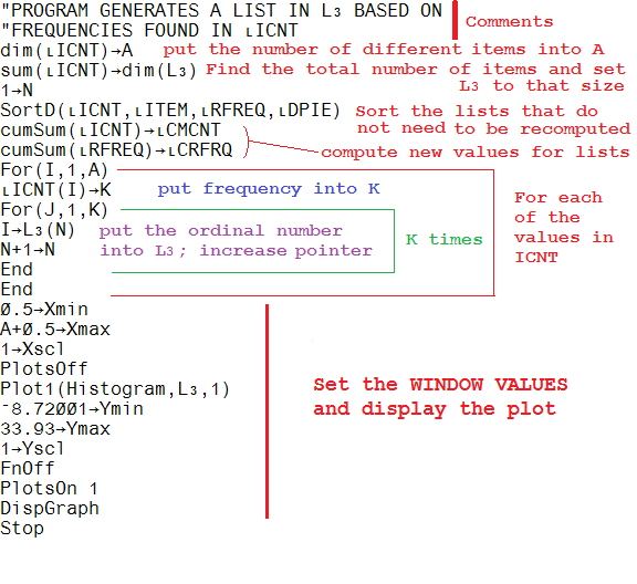
stop. So, here is an annotated listing of such a program.
Figure 30
 |
We leave Figure 29 by pressing the
keys.
|
Figure 31
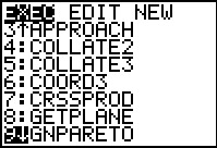 |
Press  to get the list of programs and
move down, using , to highlight GNPARETO.
Press to select that program and paste
the command onto the main screen. to get the list of programs and
move down, using , to highlight GNPARETO.
Press to select that program and paste
the command onto the main screen.
|
Figure 32
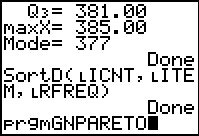 |
In Figure 32 we have the command to run the program, press
to start the program.
|
Figure 33
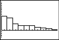 |
The program runs without any intervening output and moves directly to
a display of the graph that the program set up. This is the graph of
the data that the program put into L3.
It has exactly the correct form for the Pareto graph of the
data that we had in L1.
Remember that we used COLLATE2 to generate the required lists.
Then we run GNPARETO to produce the Pareto chart shown in Figure 33.
|
Figure 34
 |
We do need a few words of caution here. Note that if we move into
TRACE mode via the  key that the
height (n=17) of the first column is correct. However, that first
column in this chart represents the 17 "1's" that the program
placed in L3, not the 17 "377's" that
were in the original data. key that the
height (n=17) of the first column is correct. However, that first
column in this chart represents the 17 "1's" that the program
placed in L3, not the 17 "377's" that
were in the original data.
|
Figure 35
 |
While we are checking, we should look at the lists that were sorted and recreated.
To to this enter the STAT Editor. Here, in Figure 35, we see that the
values are correctly sorted.
|
Figure 36
 |
For Figure 36 we move to the right to see that the CMCNT column has been
correctly recomputed.
|
Figure 37
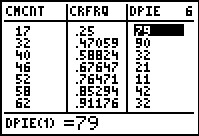 |
We move a bit further to the right and we see that the CRFRQ column is not correct.
However, there is a problem in the DPIE column. These values cannot be correct.
The largest piece of the pie must be the first one, given that this is ordered that way.
But the list in Figure 37 has the largest piece second. What went wrong?
Reviewing the program there is no obvious error. If the error is not in the
program then perhaps the error was caused by the operator, namely me. What could I have done
wrong?
The error that I made was to not strictly follow the designed pattern of use.
I wrote the GNPARETO
program to work on the output of the COLLATE2 program. We ran COLLATE2
back in Figure 4. Then we ran GNPARETO in Figure 32. However, between those
actions we went in and we sorted three of the lists back in Figure 26.
When we did that we destroyed the corresponence of the values in DPIE
with values in the other lists.
Were we to go back and rerun COLLATE2 and then run GNPARETO
we would get correct results.
|
Figure 38
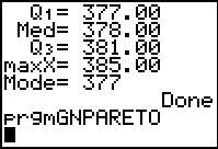 |
Figure 38 shows the main screen after rerunning COLLATE2 and GNPARETO,
and exiting the graph at the end of the latter.
|
Figure 39
 |
Figure 39 shows the start of the display of the resulting lists.
|
Figure 40
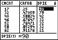 |
Figure 40 shows the top of the other lists. We see that the
LDPIE list is now correct.
|