Figure 1
|
Problem Statement:
From a population with a known standard deviation of 2.76,
we draw a sample of size 52 and from that sample we get a
sample mean=–22.8. Find the 95.0% confidence interval
for that statistic. (Express answer rounded to 3 decimal places.)
(Answer: –23.550 ≤ x ≤ –22.050)
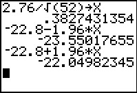
Knowing the population standard deviation means that we can
use the normal distribution tables. We know that the standard devaition of the sample means will be approximately
`sigma/sqrt(n) = 2.76/sqrt(52)`.
We calculate this value and store it in `X`.
We also know, or we could look up or compute, that the z-score corresponding to
`95%` is `1.96`. Therefore, our confidnece interval will be the interval
from `barx-1.96*2.76/sqrt(52)` to `barx+1.96*2.76/sqrt(52)`.
On the calculator we compute these values as
–22.8–1.96*X
and
–22.8+1.96*X
|
Figure 2
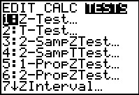 |
An alternative approach is to use the built-in ZInterval command.
We find this command on the STAT menu, over under the TESTS
sub-menu. For the calcualtor used to generate Figure 2, this is item 7.
Press  to move to Figure 3. to move to Figure 3.
|
Figure 3
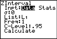 |
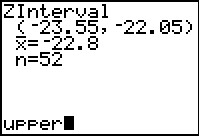
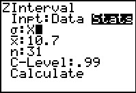
The ZInterval command bring up the screen shown in Figure 3.
THe command has two modes of operation. In the DATA mode we just
need to supply the underlying population standard deviation and the actual sample items, along
with specifying the desired confidence intreval. We do not have data to do this.
Rather we want to use the Stats mode where we supply the required statistics from the sample.
|
Figure 4
 |
To change to Stats mode move the cursor to the right to highlight "Stats"
and then press  .
Once we have done that the rest of the screen changes. We will need to
supply values for these fields. .
Once we have done that the rest of the screen changes. We will need to
supply values for these fields.
|
Figure 5
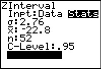 |
In Figure 5 we have supplied the underlying standard deviation
(the value for `sigma`), the sample mean (the value for `barx`), the sample
size (the value for `n`), and the confidence interval level (the value for C-Level).
Then we move the cursor to the Calculate command at the bottom of the
form.
Once that is highlighted we press to perform
the command usig the supplied values. This produces Figure 6.
|
Figure 6
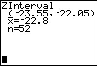 |
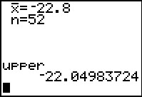
The output from the ZInterval command gives us the desired interval as well
as displaying the sample mean and the sample size.
Comparing the results shown here and the results of our calculations in Figure 1
we note that our earlier work gave many more digits to our answers than we get from the
display shown here. This raises the question of how we can get more digits shown here.
There is a simple answer to that, we can't do it. But we can "find" and "display"
the longer versions of the values shown here.
|
Figure 7
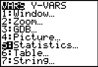 |
To do this we first move to the VARS menu. Then we move to the Statistics...
option.
|
Figure 8
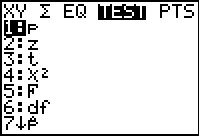 |
Once we are at the Statistics... screen we move the highlight to the right
to display the TEST sub-menu.
The items we want are way down on this list.
As we see, at the moment the highlight is on the first item.
The easiest way to get to the items we want is to press the
 key. That will take us to the bottom of the list,
shown in Figure 9.
use key. That will take us to the bottom of the list,
shown in Figure 9.
use
|
Figure 9
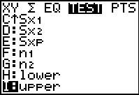 |
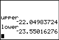
The two items at the bottom of the list, lower and upper,
hold the lower and the upper values in the confidence interval. At the moment
the last item, upper, is highlighted. We press
to paste that onto the main screen.
|
Figure 10
 |
Here we see that upper has been pasted tot he main screen. Press
and the calcualtor will display the value stored in upper.
|
Figure 11
 |
Here is the much longer version of the upper side of the confidence
interval that the calculator found back in Figure 6.
|
Figure 12
 |
We could go through that whole process again, going to the VARS
menu, the Statistics... option, the TEST sub-menu, and then move to the bottom
of the list and move up one to highlight lower. Then press
to paste that onto the main screen. Then press to get the value stored in
lower. The result is shown in Figure 12.
Thre are just too many steps that we need to take to display the values of
lower and upper. However, we will probably want to get these
values fairly often. This is the perfect situation for us to write a really short
program that will display these values.
The program we want would have jsut two lines:
Disp "LOWER",lower
Disp "UPPER",upper
We will create this in Figures 13 through 21.
|
Figure 13
 |
Use  to open the PRGM menu.
Then use to open the PRGM menu.
Then use  to highlight the NEW option. We do want to create a new program
so we press .
to highlight the NEW option. We do want to create a new program
so we press .
|
Figure 14
 |
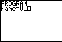
The first thing we need to do is to give the program a name.
The calcualtor is already in alphabetic mode.
Press   to generate the UL name shown in Figure 15.
|
Figure 15
 |
Press to complete the
process.
|
Figure 16
 |
We are now ready to write the lines of the program.
|
Figure 17
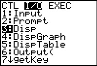 |
Press and
to move to the I/O program choices. Then move down to
highlight the Disp command. Press
to select that command.
|
Figure 18
 |
The command is placed onto the program edit screen.
|
Figure 19
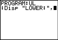 |
To continue forming our first line we press
  to "lock" the alphabetic mode. Then we press
 to generate the quotation mark, followed by to generate the quotation mark, followed by
 
 to generate LOWER,
then for the closing quotation mark.
Then we press
to exit alphabetic mode. To complete Figure 19
we press to generate LOWER,
then for the closing quotation mark.
Then we press
to exit alphabetic mode. To complete Figure 19
we press  to generate the comma. to generate the comma.
|
Figure 20
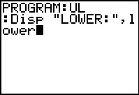 |
We want to append the name lower to complete the command, but we cannot type in
such lower case letters. Instead we need to get the name
the same way we did back in Figure 11. That is, we press
 to get to the VARD menu.
Then we go to the Statistics... option via the
key. Then we move to the
TEST sub-menu where we find, at almost the bottom of the list the
name lower. We highlight that name and
press . This pastes the name into the program editor.
To complete the line we press
and move to FIgure 21. to get to the VARD menu.
Then we go to the Statistics... option via the
key. Then we move to the
TEST sub-menu where we find, at almost the bottom of the list the
name lower. We highlight that name and
press . This pastes the name into the program editor.
To complete the line we press
and move to FIgure 21.
|
Figure 21
 |
For Figure 21 we go through the same process again to
get the Disp command from the PRGM menu under the I/O
sub-menu, then move to alphabetic mode to enter "UPPER".
Then exit that mode and append the comma. Finally, return to the VARS
menu and find upper at the end of the TEST sub-menu
which we get to through the Statistics option.
Finally, we end the line with .
At this point the program is doen. we
paress  to leave the progeram editor and return to the main screen.
|
Figure 22
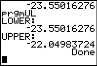 |
From the main screen we return to the PRGM menu
and select the UL program. This pastes the command
prgmUL onto the screen.
will run the program.
The program output is exactly the valeus we want.
This is a good deal of work to build the program, but now that it is on
this calculator any time that we want to get see the full values of the
calculated lower and upper bounds for a confidence interval
all we need to do is to run the program.
|
Figure 23
 |
Problem Statement:
From a population with a known standard deviation of 0.85,
we draw a sample of size 46 and from that sample we get a
sample mean=36.4. Find the 80.0% confidence interval for
that statistic. (Express answer rounded to 3 decimal places.)
(Answer: 36.239 ≤ x ≤ 36.561)
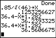
Again, the standard deviation of the sample means is given as
`sigma/sqrt(n)`, which in this case is `.85/sqrt(46)`, a value that we compute and then store in X.
We know, from looking it up on a table or from computing it separately, that the z-score
associated with having 90% of the normal distribution to its left
is 1.282. That means that there is 10% to the right of
z=1.282. It also means that there is 10% to the
left of z=–1.282. Therefore,
our 80% confidence interval runs from
`36.4-X*1.282` to `36.4+X*1.282`.
We see the answers in Figure 23.
|
Figure 24
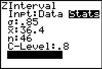 |
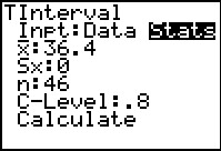
Again, we could have let the calculator do all of the work for us by
using the ZInterval command.
Recall from Figure 2 that we can find the ZInterval
command via  to open the STAT
menu. Then we need to move tot he
TESTS sub-menu. When we highlight and select
the ZInterval option the calculator responds
by displaying the input form shown in Figure 24. Here we
enter the values for `sigma` (in this case that would be .85),
for `barx` (in this problem that is 36.4), for `n` (here we have samples of
size `46`), and the desired C-Level (this problem asks for the
80% confidence interval). Then, as shown in Figure 24,
we move to the Calculate field and press . to open the STAT
menu. Then we need to move tot he
TESTS sub-menu. When we highlight and select
the ZInterval option the calculator responds
by displaying the input form shown in Figure 24. Here we
enter the values for `sigma` (in this case that would be .85),
for `barx` (in this problem that is 36.4), for `n` (here we have samples of
size `46`), and the desired C-Level (this problem asks for the
80% confidence interval). Then, as shown in Figure 24,
we move to the Calculate field and press .
|
Figure 25
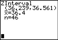 |
The result is shown in Figure 25. Again, the values shown for the lower
and upper limits to our confidence interval
are somewhat limited in the number of digits displayed.
However, we now have the UL program to help us with this.
|
Figure 26
 |
We can run the UL program and it displays the calculated valeus
for the
lower
and upper limits to our confidence interval.
|
Figure 27
 |
Problem Statement:
From a population with a known standard deviation of 5.73,
we will draw a sample. We will use the generated sample mean
to produce a confidence interval.What is the smallest
sample size that will produce a 99.0% confidence interval
that has a margin of error ≤ 1.9?
(Answer: 61)
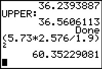
Because we know the population standard deviation, the margin of
error, which we can call `m`, for a 99% confidence interval
is given by `m = (z_(.995))*sigma/sqrt(n)`.
We can transform this to be `sqrt(n) = (z_(.995))*sigma/m`, or
`n = ((z_(.995))*sigma/m)^2`. Using the values in this problem
that becomes (5.73*2.576/1.9)².
The answer, `60.35229081`, gives the value of `n` that we need
for equaltiy in the equation, but we cannot have `60.35229081`
items in a sample. Sample size needs to be a whole number.
We need to round up the answer to the next higher whole number,
in this case, 61.
|
Figure 27a
 |
Problem Statement:
From a population with an unknown standard deviation we draw
a sample of size 31 and from that sample we get a sample
mean=15.2 and a sample standard deviation=2.02.
Find the 98.0% confidence interval for those statistics.
(Express answer rounded to 3 decimal places.)
(Answer: 14.309 ≤ x ≤ 16.091)
We do not know the population standard deviation.
Therefore, we need to use the sample standard deviation as an
approximation to the population standard
deviation. However, in that case, we also have to shift from
using the normal distribution to using the Student's t
distribution
of the sample mean.
Just as was the case for the normal distribution, to find the 98%
confidence interval, we need to find the value, in this case the t-value
rather than the z-score,
that has 99% of the area under the Student's t curve to the
left of that point. With a normal distribution we would use
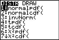
the invNorm( command to find such a z-score.
The image in Figure 27a is from a TI-83 Plus, although it could have been
from a TI-84 Plus running the early 2.21 operating system.
The important thing to notice in this page is that there is no
corresponding invT( option available. Therefore,
on the older calculators we cannot directly ask for the desired
Student's t value. [In Figure 28 we will look at program
for the earlier calculators that gets this value for us.]
|
Figure 27b
 |
The image in Figrue 27b was taken from a TI-84 Plus running more recent software.
Now the DIST menu includes the invT( option.
We select that option and
have it pasted to the main screen.
|
Figure 27c
 |
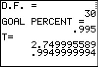
For invT( command requires us to provide the proportion of the
area to the left of the desired point and the number of degrees of freedom for the request.
We want 99% and, for a sample size of 31 we have 30 degrees of freedom.
The calculator produces the desired Student's t value of
2.457261531.
|
Figure 28
 |
In Figure 28 we start the INVT program. This is a slow program that produces
results similar to, but not exactly the same as, the invT(
command on the newer calculators. The results are quite close, certainly
close enough for our needs. Any computation with more than
2 degrees of freedom should produce results that are accurate to at least 4 decimal places.
With 1 or 2 the degrees of freedom the t-values may
not be quite as close, but the
difference in the area under the curve for the two values is near 0.
|
Figure 29
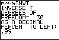 |
Figure 29 shows the input for the progrram.
|
Figure 30
 |
Figure 30 shows the calculated results. Compare the program
result of
t=2.457261443 to the invT result from Figure 27c of
t=2.457261531. The difference is there but beyond our needs.
Tables of Student's t values generally give those values to at most
4 digits. Thus, looking up the value in a table would produce 2.457.
|
Figure 31
 |
Restate the problem:
From a population with an unknown standard deviation we draw
a sample of size 31 and from that sample we get a sample
mean=15.2 and a sample standard deviation=2.02.
Find the 98.0% confidence interval for those statistics.
(Express answer rounded to 3 decimal places.)
(Answer: 14.309 ≤ x ≤ 16.091)
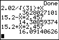
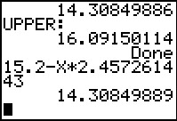
Now that we have a t value for the 98%
confidence interval, we just need to compute the margin of error
`t_(1-alpha/2)*s_x/sqrt(n)` or in our case `2.457*2.02/sqrt(31)`.
Figure 31 shows the computation of the lower and upper bounds of the confidence
interval.
Note that the values computed here used
the table t-value of 2.457.
This will make our endpoints for the confidence interval slightly
different than if we had used either of our longer values from above.
|
Figure 32
 |
As before, we could have just let the calcualtor do all the work.
Althought eh older calculators did not have the invT(
command, all of the calculators have the
TInterval... command in the TESTS sub-menu of the STAT
screen.
We move to and select that TInterval... command.
|
Figure 33
 |
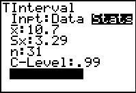
The result is the input form shown in Figure 33.
Again we want to be sure that we are in the Stats mode on this
screen.
Then we proceed to supply the calculator witht he required values.
|
Figure 34
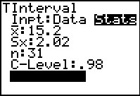 |
We have placed the problem values in the appropriate spots.
Having highlighted the Calculate field, press
to perform the computation.
|
Figure 35
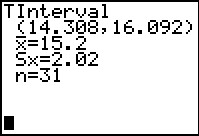 |
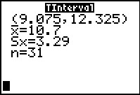
The interval is displayed.
The longer version of the interval endpoints has been stored in
lower and upper.
|
Figure 36
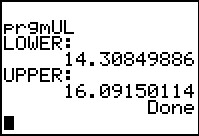 |
Our UL program displays those longer values.
Comparing those values to the ones that we found in Figure 31
we see that they are slightly different.
Again, the Figure 31 values came from using the t-value
of 2.457, whereas these values came from using the calculator
determined t-value, shown back in Figure 27c as
2.457261531.
|
Figure 37
 |
Were we to redo the computation using the value from the INVT
program, from Figure 30, namely, 2.457261443, we
would get the value shown in Figure 37. The results are quite close.
|
Figure 38
 |
Problem Statement:
From a population with an unknown standard deviation
we draw a sample of size 31 and from that sample we get a
sample mean=10.7 and a sample standard deviation=3.29.
Find the 99.0% confidence interval for those statistics.
(Express answer rounded to 3 decimal places.)
(Answer: 9.075 ≤ x ≤ 12.325)
To do this in the way that we would by hand, we first need to find the
required t-value
for a 99% confidence interval with 30 degrees of freedom.
For Figure 38 we have chosen to run the INVT program to get that value.
|
Figure 39
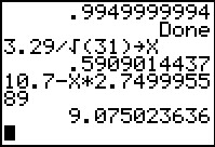 |
Figure 39 uses that value and the values supplied in the
problem to compute the lower end of the confidence interval.
|
Figure 40
 |
Figure 40 uses the t-value from Figure 38
and the values supplied in the
problem to compute the upper end of the confidence interval.
|
Figure 41
 |
For Figure 41 we return to using the power
of the calculator via the TInterval command.
Here we have entered the values from the problem.
|
Figure 41a
 |
The results conform to the values that we obtained earlier.
|
Figure 42
 |
Problem Statement:
We have a population of 678 members.
Each member has one of two characteristics, S or T.
We have a sample of this population and in that sample
we find 15 members with S and 14 members with T.
Build and state a 90.0% confidence interval for the proportion of characteristic S from this sample.
(Give your answer rounded to 3 decimal places.)
(Answer: 0.365 ≤ p ≤ 0.670)
To do this problem the long way we first compute the standard deviation
of the sample proportions.
15/29 is the proportion of characteristic S
in our sample.
`sqrt((P*(1-P))/29)` is the standard deviation of the sample proportions.
Such sample proportions are normally distributed. Therefore, for a
90% confidence interval we use the z-score of 1.645.
Our lower end of the confidence interval will be .3645977959.
|
Figure 43
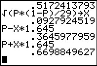 |
The upper end of the confidence interval is
.6698849627.
|
Figure 44
 |
Of course, once we know the standard deviation of the sample proportions,
we could have had the calcualtor do the rest of the
work by using the ZInterval command.
Here we have used that command to bring up its input screen.
We are about to specify the standard deviation. Rather than type the value that
we found earlier we will just reference it by using the variable X,
the place where we stored the standard deviation computed in Figure 42.
|
Figure 45
 |
The calculator places the stored value of X onto the screen.
Now we will put the proportion, P, into the value of `barx`.
|
Figure 46
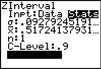 |
Again, the calculator fills in the needed value.
Note that we set n to be 1.
Then we set the C-Level to be the specified .9.
|
Figure 47
 |
After telling the calulator to Calculate the result it displays
Figure 47 with essentially the same values that we obtained above.
The difference will be due to the fact that the
ZInterval command uses the fully computed z-score for
a 90% confidence interval, not the 1.645
table value that we used
back in Figures 42 and 43.
|
Figure 48
 |
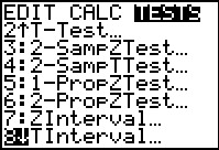
As one might expect, there is an even shorter route to the same answer.
In the TESTS sub-menu of the STAT screen,
there is a command 1-PropZInt that will just do the problem.
We find and highlight that command, then press
to execute it.
|
Figure 49
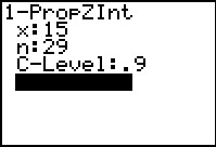 |
The command brings up an inout screen.
We just need to supply the values.
The x value is the number of items with the desired characteristic.
The n is the sample size.
C-Level is the confidence interval expressed as a decimal.
The final field is Calculate.
Press to do the computation.
|
Figure 50
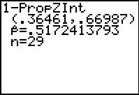 |
Figure 50 shows the result, identical to the work we did earlier in Figure 47.
|