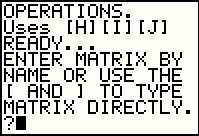
 key to get to the MATRIX
screen. The TI-83 Plus and TI-84 Plus calculators use the two key sequence
key to get to the MATRIX
screen. The TI-83 Plus and TI-84 Plus calculators use the two key sequence

 to get to the MATRIX
screen. The results of the calculator survey for the Fall 2010 semester are:
to get to the MATRIX
screen. The results of the calculator survey for the Fall 2010 semester are:
IMPORTANT NOTE: The TI-83 uses the key to get to the MATRIX
screen. The TI-83 Plus and TI-84 Plus calculators use the two key sequence
to get to the MATRIX
screen. The results of the calculator survey for the Fall 2010 semester are:
 to demonstrate moving to the
MATRIX screen. Users of tthe TI-83 will have to substitute their one key action for the two key presented here.
to demonstrate moving to the
MATRIX screen. Users of tthe TI-83 will have to substitute their one key action for the two key presented here.
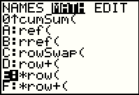
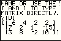
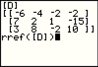
Entering and editing data in a matrrix is covered in Figures 1 through 36 of the Matrix Entry, etc. page. Review that page if you have any questions about creating, loading, or changing a matrix. Also, although that page creates a matrix in [D], this page starts at a point where a different matrix has been loaded into [D]. That matrix, the one assumed to be stored in [D] at the start of this page, is shown in Figure 1 below.

|
Somehow or other, matrix [D] has been specified as having 3 rows and 4 columns,
and the values shown in Figure 1. Displaying [D] as we have done in Figure 1 also makes
the value of [D] be the current value of ANS, the most recent "answer". We note that
it is the value that was displayed, not the actual matrix [D] that is stored in
ANS. If we use ANS in a calculation we are using its current value, not the
matrix that gave it that value. More will be said later on this.
Goal: Rather than just perform arbitrary elementary row operations as a way of demonstrating them, we want to approach this demonstration with a goal in mind. We will aim to transform matrix [D], using just the elementary row operations, into a form where each matrix entry on the main diagonal will be a 1 and where all of the entries above and below that main diagonal have the value 0. Values in the final column will just be as they are computed. It is not the purpose of this page to discuss the the reason for having this goal or even the interpretation of the results. At this point, it is just a goal. We arrive at that goal in Figure 22. Feel free to look ahead if you need a clarification of the goal. |
 |
The first step is to get a 1 in the first row, first column
posiiton. THere are a number of different ways to
do this. In this case we have chosen to
add the contents of row 2 to the contents of row 1.
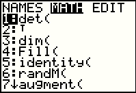
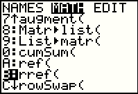
We can find the command to do this by moving to the MATRIX window
and then using the  key to move to the MATH subwindow,
as shown in Figure 2. There we see a list of the commands available in this subwindow.
Unfortunately, the one we want, row+(, is not in the list. However, we note,
by the fact that there is a down arrow at the last item in the screen, that there are more
options. We use the key to move to the MATH subwindow,
as shown in Figure 2. There we see a list of the commands available in this subwindow.
Unfortunately, the one we want, row+(, is not in the list. However, we note,
by the fact that there is a down arrow at the last item in the screen, that there are more
options. We use the  key to move
the highlight down until we reach our desired command, or until the command is on the screen. key to move
the highlight down until we reach our desired command, or until the command is on the screen.
|
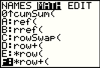 |
Figure 3 shows that we have gone beyond the desired command. We press the
 key to select
item "D:row+( "
to paste onto our primary screen. key to select
item "D:row+( "
to paste onto our primary screen.
|
 |
Figure 4 shows that the row+( command was indeed pasted onto the screen,
and we complete the
command by pressing  to insert
Ans to indicate that we want the command to operate on the
matrix stored in Ans, to insert
Ans to indicate that we want the command to operate on the
matrix stored in Ans,
  to indicate that we want to add the contents of row 2,
 to the contents of row 1, and to the contents of row 1, and
 to complete the command. Then we press to complete the command. Then we press
 to perform the command. The result is displayed
in Figure 4. to perform the command. The result is displayed
in Figure 4.It is important to recognize that the result, shown in Figure 4 at the bottom is not only displayed but also is now the current value of Ans. Furthermore, nothing has changed in [D]. |
 |
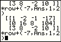
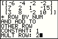
Our next task is to take the values below our row 1, column 1 value and make those all zero.
We can use the *row+( command to do this. We want to multiply -7 times row 1 and add those values
to row 2. Remember that we are working on the version of the matrix
that is stored in Ans. Reading the TI description of the command given above,
we formulate the command shown below in
Figure 6, namely *row+(-7,Ans,1,2). First we want to find the
command. We look in the MATRIX window and then at the CALC subwindow
to find our desired command. Figure 5 shows the end of the list of commands.
Because the desired command is highlighted, we press the
key to paste that command onto the screen.
|
 |
Figure 6 not only shows the pasted *row+( command, but also
Figure 6 shows the completion of the command, via
 followed by
to get Ans
pasted on the screen, and ending with
followed by
to get Ans
pasted on the screen, and ending with
 to finish composing the command, and
to perform the command.
The calculator works uses the old value of Ans, does the elementary
row operation as instructed, and produces the
new matrix, now the current value of Ans, shown at the bottom of Figure 6 to finish composing the command, and
to perform the command.
The calculator works uses the old value of Ans, does the elementary
row operation as instructed, and produces the
new matrix, now the current value of Ans, shown at the bottom of Figure 6
|
 |
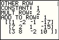
Our next command is meant to produce a 0 to replace the 3 in row 3 column 1.
We want to use the *row+( command to do a -3 times the first row and
add it to the third. Rather than go through the process
of entereing the command, we will
press the keys to recall the previous
command. That is how we generated the com,mand at the bottom of Figure 7.
Note that we have just recalled the command, not performed it. Before we perform it
we will use the cursor keys to move around
in that command so that we can make changes to it.
|
 |
Figure 8 shows the modified command where we changed the -7 to -3 and altered
the receiving row from 2 to 3. Having modified the command, we
press the key to perform the command.
|
 |
Figure 9 shows the results of the previous command. Our next challenge is to change the item in row 2 column 2 to be 1. To do this we can use another elementary row operation, row*(, which allows us to multiply a row fo the matrix by a constant. We cannot recall that command because we have not used it recently. Instead, we return to the MATRIX window in Figure 10. |
 |
Here we have not only returned to the MATRIX window, we have also moved
to the MATH subwindow and then moved down that window so that we have
highlighted the row*( option. We use the
key to select that option and paste it onto out main screen.
|
 |
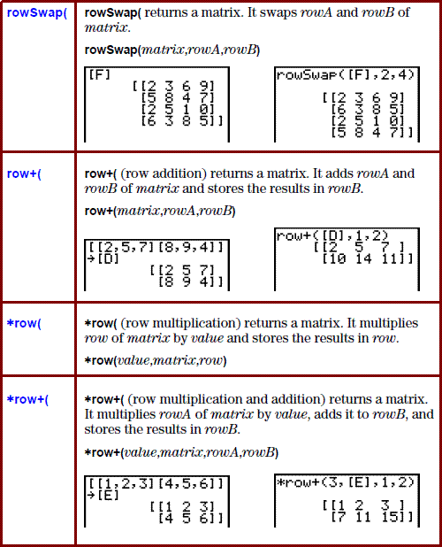
To complete Figure 11 we consult the chart above Figure 5 to see the
syntax of the row*( command. We see that we need to provide value
used to multiply a row, the name of the matrix, and the number of the row that we want to use.
Therefore we complete the row*( command with 1/16,Ans,2).
Finally, we use to perform the command.
The result is shown in at the bottom of Figure 11.
|
 |
Figure 11 is the first time that we have seen a decimal value in the matrix. There is nothing wrong
with this, although at times we would prefer to see the fraction designation for
such values. We can do this by using the  key to
open the MATH window shown in Figure 12. The option that we want is the first one, key to
open the MATH window shown in Figure 12. The option that we want is the first one,
 . That happens to be highlighted. We use the
key to paste symbol onto the
screen. . That happens to be highlighted. We use the
key to paste symbol onto the
screen.
|
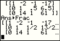 |
Notice, in the middle of Figure 13, that the calculator automatically inserted the
Ans before the . We followed that command
with the key.
The calculator responded by repeating the value of Ans
but this time with values in fractional form where needed.
|
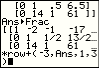 |
The next task is to use the 1 that we just created in row 2 column 2 to change the value below it to
0. To do this we want to multiply row 2 by -14 and add that to row 3. We start by recalling
commands (repeating the sequence)
until we have recalled a *row+( command, as shown in Figure 14.
|
 |
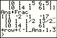
Figure 15 shows that we have changed the -3 to -1 and we have
the cursor sitting on top of the comma
that rests between the -3 and Ans. We need to get a 4 in there
to make the desired -14. We can move to INSERT mode
by pressing  . This changes the
display to that seen in Figure 16. . This changes the
display to that seen in Figure 16.
|
 |
In Figure 16 we see that the cursor flashing black square has been replaced by a flashing underscore. This indicates that we are INSERT mode. |
 |
Now we press the  key to insert the desired 4, and then we can use the
cursor key, , to move to the right where we can
change the 1 of the old command to the 2 that we desire.
After making these changes we press the key to
get the calculator to perform our
modified command. key to insert the desired 4, and then we can use the
cursor key, , to move to the right where we can
change the 1 of the old command to the 2 that we desire.
After making these changes we press the key to
get the calculator to perform our
modified command.
|
 |
The command is performed, the new Ans is displayed. Our next step is to change the -6 that is in row 3 column 3 to be a 1. We can do that by multiplying the third row by -1/6. We have recalled the command to muliply a row by a value, and we have changed that recalled command to suit our current needs. |
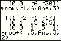 |
As of Figure 19 we have 1's down the main diagonal and everything beloww that is a 0. We continue the process by changing the values above row 3 column 3 to be 0. The value .5 above row 3 column 3 needs to be changed. The *row+( command will do this. We merely need to multiply row 3 by -0.5 and add the result to row 2. The command to do that has been recalled and modified at the bottom of Figure 19. |
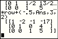 |
Performing the command at the bottom of Figure 19 yields Figure 20. Our next step will be to change the -1 in row 1 colum 3 to 0. We can do this with yet another *row+( command, as shown in Figure 21. |
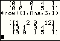 |
One more *row+( command will be needed to clear out the -2 in row 1 column 2. |
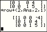 |
Here we not only see that final command, we also see the completed reduced row echelon form of the matrix. |
The steps shown above moved us from the initial statement of the matrix [D]
to our goal matrix, 1's down the main diagonal and 0's above and beow that diagonal.
The process works. The elementary row operations
are all that we need to do this.
There are three difficulties however.
First, we need to remember the format for the various elementary row operations,
at least until we can get to the point where we can recall earlier successful
examples. Second, if we make a mistake it is going to be hard to recify that error.
And, third, we are using the value in Ans throughout the process. In fact, there are a number
of times when we needed to key in the Ans symbol via the
keys.
All of this means that there is a bit of a challenge to this process.
The Figures below demonstrate a possible aid to this issue in the form of a
program, ELROWOPS, that manages our
elementary row operations. We will solve th same probblem, but this time
via the ELROWOPS program.
|
|
Figure 23 merely restates Figure 1. We started with a matrix in [D] and we used the initial value of that matrix, as stored, modified, and represented in Ans, during the entire process from Figure 1 through Figure 22. |
 |
Using the  key we open the window shown in Figure 24.
In this case we also moved the highlight down to the item holding the ELROWOPS program. key we open the window shown in Figure 24.
In this case we also moved the highlight down to the item holding the ELROWOPS program.
|
 |
The
key moves us to Figure 24 where we will press
again to actually run the program.
|
 |
Here we have the starting screen for the program.
The next program screen, in Figure 27, warns us that this program will make use of the matrices
[H], [I], and [J]. This is a warning in case we had
stored some values in those matrices. Using this program would probably destroy,
that is overwrite, anything that we had previously stored in those matrices.
Press to continue.
|
 |
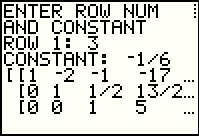
The program prompts us for the starting matrix. We could type it in or, if we already entered it and have it stored in a matrix, we can simply provide the name of the matrix. |
|
|
left blank... |
 |
Using the sequence we open
the MATRIX window. Then we can move to highlight the [D]
matrix, the name we want to paste onto our main screen.
The key moves us to the main screen where the
calculator has indeed pasted the [D] matrix name.
|
 |
We are ready to go forward. Press to
have the program accept the matrix name.
|
 |
The program displays the matrix and then waits
for our signal to go forward.
We know that we want to multiply row 2 by 1 and add it to row 1.
Press to move to Figure 32 where the program gives us a list of
possible actions.
|
 |
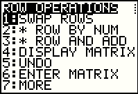
Item 3 in our menu is the operation we want. Press  to select that item and its asscoiated action.
|
 |
The program reminds us of what it is about to do (Multiply a row by a number and
add that to another row.) and then the program asks for the constant value. We respond
with .
The program accepts this and asks for the row to multiply.
We respond with . That is the state illustrated in Figure 33.
|
 |
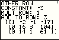
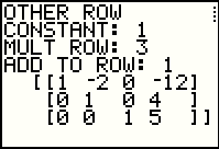
We continue with to accept the response given at the end of Figure 33.
The program now asks for the row to which we are to add the values.
We respond with .
The program then performs the desired elementary row operation
and follows that by displaying the result. The program pauses so that we can study
the result. When we are ready to continue
we press to move back to the menu shown in Figure 35.
Before we do that we want to plan our next move. That will be to multiply
-7 time row 1 and add the result to row 2.
|
 |
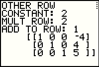
We are back at the program menu. Again we choose item 3. |
 |
Figure 36 displays the resul of our responding to the
prompts for item 3 of the menu. You can see, in Figure 36, that we told the program to
use the constant -7, to multiply
the constant times row 1, and to add the result to row 2.
The outcome is as we would expect, and again, the program is waiting for us to give it the
OK to return to the menu.
We plan our next move, multiply row 1 by -3 and add the result to row 3.
With that plan in mind, we press to return to the menu
where will again select item 3. Rather than re-display the menu at each step, the following
Figures merely show the sequence of commands.
|
 |
Here we see that we did specify multiply row 1 by -3 and add it to row 3. The resulting matrix follows. |
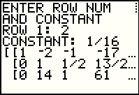 |
Here we have responded to a different command, menu item 2, and we have indicated that we wish to multiply the contents of row 2 by 1/16. |
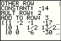 |
Return to menu item 3 to multiply -14 times the contents of row 2 and add the result to rwo 3. |
 |
Now we do another row multiply, this time telling the program to multiply row 3 by the constant -1/6. |
 |
Multiply -1/2 times row 3 and add to row 2. |
 |
Multiply 1 times row 3 and add to row 1. |
 |
Multiply 2 times row 2 and add to row 1.
We are really done at this poitn. The program is waiting for
us to pess to return to the menu.
When we do press that key we are returned to the menu which will be as shown in Figure 35.
There we note that item 7 of the menu gives you more menu choices.
We will take that option.
|
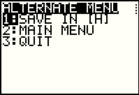 |
This is the second menu. It has limited choices, but we are done so
we will
simply press the key to move to Figure 45.
|
 |
Strangely enough, the program responds by displaying the word QUIT.
However, the program is not really done. We can tell that we are still in the
program because we continue to get the little dots at
the upper right edge of the screen. The program is still waiting for us to respond with
the key.
|
 |
When we do that the program finally ends, the calculator displays Done, and we are returned to our usual cursor. |
Thus far, in Figures 1 through 22, we have applied elementary row operations to transform matrix [D] into the desired form. Then, in Figures 23 through 46, we did the same thing using the ELROWOPS program to manage and facilitate our work. We took the same steps the second time, but we did so through the menu and prompts of the program. The process used to make the transformation is so formulaic that we can apply the algorithm to other matrices to get a similar transformation. It is often the case that we want to get the reduced row echelon form of a matrix. Even with the help of the ELROWOPS program, this is a long process. Fortunately, the TI-83 family of calculators provides a single command to do all of the work for us. This is the rref( command.
|
|
Just to refresh our memory, we
return to the MATRIX window and select [D]
to paste it onto our main screen.
Then press the key to get the display in
Figure 47.
|
 |
In Figure 48 we have returned to the MATRIX window, moved to the MATH
subwindow, and then moved down the list of options until
we can find and highlight the rref( option.
We select that highlighted option
by pressing the key.
|
 |
The calculator responds by pasting the command onto the main screen. |
 |
To complete the task we need to return to the MATRIX window and again select
[D] to paste it onto the main screen. Then we complete the command with a closing parenthesis..
Press to instruct the calculator to perform the command.
|
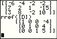 |
The result, shown in Figure 51, is the reduced row echelon form of the matrix. Thus, in one command we had the calculator do all of the work that we did step by step either through the direct use of elementary row operations or via the use of the ELROWOPS program as an intermediary to perform those same operations. |
©Roger M. Palay
Saline, MI 48176
February, 2013