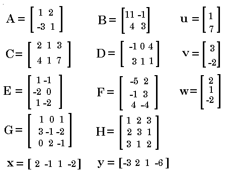
IMPORTANT NOTE: The TI-83 uses the key to get to the MATRIX screen. The TI-83 Plus and TI-84 Plus calculators use the two key sequence to get to the MATRIX screen. This page will consistently use the two key sequence to demonstrate moving to the MATRIX screen. Users of tthe TI-83 will have to substitute their one key action for the two key presented here.

Figure 1	First, we move to the MATRIX window to see that the matrices are in the calculator, at least with respect to the rows and columns. [See the note above for methods of entering the desired matrices if need be.]
Figure 2	Figure 2 shows the contents of [A] and [b]
Figure 3	Select [A] from the MATRIX window, then , select [B] from the MATRIX window, and then press to perform the command. The resulting matrix is shown in Figure 3.

We need to stop here and examine the result of the multiplication of two matrices. The resulting answer is not as clear as it was for matrix addition, subtraction, scalar multiplication, or a combination of these. To perform a matrix multiplication each element of the answer is formed by obtaining the sum of the products of the elements of the corresponding row of the left matrix with the elements of the corresponding column of the right matrix. In Figure 3, the 5 in the answer is in row 1 column 2. Therefore, the 5 came from adding up the products of multiplying each element of row 1 of the left matrix, [A], with each element of column 2 of the right matrix, [B]. The first row of [A] was 1  2. The second column of [B] was -1  3. We multiply 1*(-1) and 2*3, to get -1 and 6, which we add to get 5, the element in row 1 column 2 of the answer. This process is pictured for all 4 positions of the answer in the next figures.

Figure 4	Multiply row 1 of [A] times column 1 of [B] to get row 1 column 1 of the answer.
Figure 5	Multiply row 1 of [A] times column 2 of [B] to get row 1 column 2 of the answer.
Figure 6	Multiply row 2 of [A] times column 1 of [B] to get row 2 column 1 of the answer.
Figure 6a	Multiply row 2 of [A] times column 2 of [B] to get row 2 column 2 of the answer.

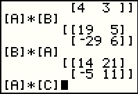Figure 7	Matrix multiplication is full of surprizes. First, note that matrix multiplication is not commutative. if we have two numbers, a and b, we know that a * b = b * a. This is called the commutative property of multiplication for real numbers. Figure 7 shows the results for [A] * [B] and then for [B] * [A], and the two answers are decidely not the same. Therefore, the multiplcation of matrices is NOT commutative. Remember that to add two matrices they have to have the same dimensions. The bottom of Figure 7 tells the calculator to multiply [A], a 2 x 2 matrix, times [C], a 2 x 3 matrix.
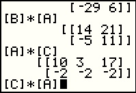Figure 8	Interestingly enough, the calculator does the multiplication and produces a 2 x 3 result. The multiplication method for matrices ties entries in the answer to corresponding rows of the left matrix and corresponding columns of the right matrix. Each of the 6 entries in the result shown in Figure 8 have a corresponding row in [A] and a corresponding column in [C]. Furthermore, the length of each row in [A] (which is given by the number of columns in [A], is exactly equal to the length of each column in [C] (which is given by the number of rows of [C]). Figure 8 ends with the formulation of a command to multiply [C] * [A]. That command results in an error as shown in Figure 9.
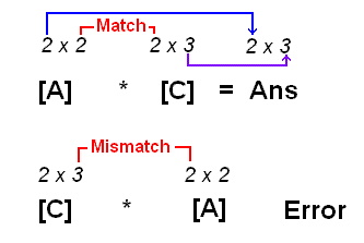
Figure 9	The error message is short: DIM MISMATCH. In this case, because we wanted to do a multiplication, the calculator insists that the number of entries in each row of the left matrix, [C] must match the number of entries in each column of the right matrix, [A]. However, [C] has 3 entries in each row (because [C] has 3 columns) whereas [A] has but 2 entries in each column (because [A] has but 2 rows). A diagram of this follows: In Figure 9 we have a choice of responses for the calculator. We can tell it to Quit or to Goto. We will demonstrate the former later, but to move to Figure 10 we will press to Goto.
Figure 10	Following the Goto choice of Figure 9, the calculator displays the offending command so that we may edit it. In this case we will replace the [A] with [E]. To do this press to move to Figure 11.
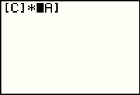Figure 11	Even though we pressed the cursor left just once, the highligh moved to the start of the [A] symbol. Remember that it is a single symbol even though it takes up the space of three characters.
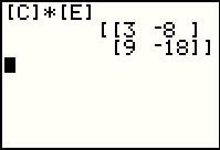Figure 12	We return to the MATRIX screen and select item 5, [E]. The calculator pastes this new symbol over the old one. Then press to perform the command. The result of multiplying [C] * [E], a 2 x 3 matrix times a 3 x 2 is a 2 x 2 matrix.
Figure 13	On the other hand, [B] * [C], a 3 x 2 matrix times a 2 x 3 is a 3 x 3 matrix. These are the results we would expect, particularly after looking at the drawing above (next to Figure 9) where we see that multiplication works if the "inner" dimensions match, and the result is a matrix with the "outer" dimensions.
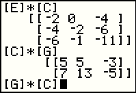Figure 14	Considering [C] * [G], the inner dimensions match ([C] has 3 columns and [G] has three rows. Therefore the multiplication should work and the result should have 2 rows (the number of rows in [C] and 3 columns, the number of columns in [G]. However, we expect the command [G] * [C] to fail because the inner dimensions do not match ([G] has 3 columns but [C] only has 2 rows.
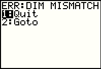Figure 15	Sure enough, the command in Figure 14 did not work. THis time we will choose the Quit option by pressing the key.
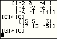Figure 16	Because we Quit in FIgure 15, the calculator leaves the offending command on the screen without performing it. The calculator is now ready for a new command.
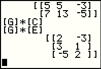Figure 17	Just to throw in one last working example here, we form the command [G] * [E], a command we do expect to work since [G] has 3 columns and [E] has 3 rows. We expect that the result will have 3 rows and 2 columns. It does.
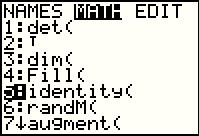
Figure 18	The multiplicative identity matrix is a square matrix with the value 1 in each entry on the main diagonal, and the zero value everywhere else. Of course we could type in or use the editor to create a multiplicative identity matrix. However, the calculator provides a nice way to generate such a matrix. We return to the MATRIX window, then move the highlight to the right one to see the MATH subwindow, shown in Figure 18. Once there we find the start of the identity( function statement as option 5, highlighted in Figure 18. IF we press to select that option, the calculator will paste the start of the command onto our screen.
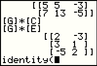Figure 19	Figure 19 has the start of the command. Now we need to finish it. All we need is the dimension of the desired matrix. It will be a square matrix, as are all identity matricess, but there is a different identity matrix for each dimension. In order to complete the command we need to specify the dimension of the desired identity matrix.
Figure 20	In Figure 20 we completed the command and had the calculator perform it. We asked for a 3 x 3 identity matrix and the calculator has created it.
Figure 21	We can demonstrate our identity matrix by using it on the left with any of the matrices that have three rows. We will use [G]. And, as expected, the product is identical to [G].
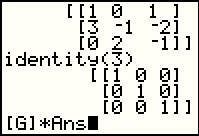Figure 22	Because [G] is a square matrix, we could multiply it on the right with the 3 x 3 identity matrix. For Figure 22 we recall the identity(3) command and perform it, then we construct the [G] * Ans command.
Figure 23	Performing the command that ended Figure 22 we see the results in Figure 23. Again, the answer is identical to [G]. In the same way we constrauct and execute a command to multiply [C] on the right by a 3 x 3 identity matrix. The result is identical to [C].
Figure 24	However, since [C] has 2 rows, the identityu matrix that we need to use to multiply on the left of [C] will have to be a 2 x 2 identity matrix, as demonstrated in Figure 24.
Figure 25	Figure 25 is a return to the MATRIX window and the MATH subwindow. In this case we want to use the augment( option.
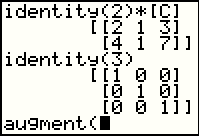Figure 26	Here we have pasted the start of the augment( function onto the screen. Now we need to supply the function with two matrices, and specifically twop that have the same number of rows. Augment will put the two matrices together to form one matrix.
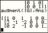Figure 27	We complete the augment( function with the matrix [G] and then Ans which held a 3 x 3 identity matrix from early in Figure 26. The result is a new matrix with 3 rows and now 6 columns.
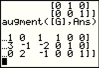Figure 28	Some of the matrix in Figure 27 was chopped off. We can use the key to move the window to the right.
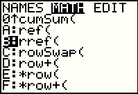Figure 29	Return to the MATRIX window, MATH subwindow, to find a then select the rref( command. Remember that rref will perform a series of elementary row operations that will turn the first m columns in an m x n matrix into having 1's down the main diagonal and 0's above and below that diagonal.
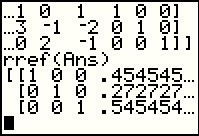Figure 30	In Figure 30 we asked that the calculator perform the rref( function on the augmented matrix that we produced earlier. The rref( function has an aim to get the main diagonal for the first 3 columns (since this has 3 rows) to be all 1's. The elementary row operations that take place to do this and to produce 0's above and below that diagonal, also change the values in the remaining 3 columns, the ones that started as an augmented identity matrix. Figure 30 can only show a bit of those new values since there is not enough room on the screen.
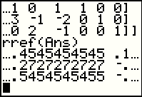Figure 31	Use the key to move the window to the right, revealing more of the exteneded values.
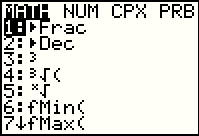Figure 32	Another approach is to use the command in the MATH menu to get the calculator to display the results in fractional form. In Figure 32 we move to the MATH menu by pressing the key. Then we can select the command by pressing the key.
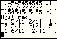Figure 33	Figure 33 shows the command after it has been pasted and executed (the calculator automatically supplied the Ans in the command). The matrix is redisplayed with the decimal values now showing up as fractions. As fractions it is easier to see more of the matrix on the screen. We still need to move the window to the right to see the rest of the result.
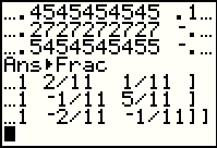Figure 34	Figure 34 displays more of the matrix.
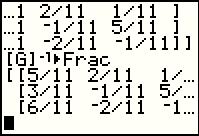Figure 35	The command in Figure 35 asks for the inverse of [G] but expressed in fractional form. We compare these values to the ones we found on the right side of the augmented matrix as displayed in Figures 33 and 34. As far as the values shown on the screen, these are the same entries.
Figure 36	Here we see the rest of the answer from Figure 35. Again, these values are an exact match for the valeus in the earlier augmented matrix.
Figure 37	Although it is a shame to waste our earlier efforts at putting a matrix into [H], because we have a small number of available matrices we will have to destroy the old contents of [H] if we want to save the matrix that we just computed, namely the value of [G]-1. Once we have stored the value in [H] we can examine [G] * [H].
Figure 38	That product is the identity matrix. Therefore, [H] is the right multiplicative inverse for [G] (because we have seen that multiplying the two matrices, with [H] on the right, yields the identity matrix). Then we formulate the command for [H] * [G].
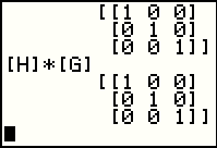Figure 39	This too yields the identity matrix. Therefore, [H] is also the left multiplicative inverse of [G]. Having seen that both products, with [H] on the left and on the right, yield the identity matrix, we can shorted the designation and just say that [H] is the multiplicative invers of [G]. And, of course, that makes [G] the multiplicative invers of [H].

The work from Figrue 26 through Figure 39 may seem a bit disconnected. Why go through that augmented matrix work followed by the application of the rref( command, if we can just get the desired values using the key as we did in Figure 35?

The answer to that is more historical than mathematical. To some extent it is the same reason that we teach and learn the elementary row operations even though rref( is available to us. There was a time when, in order to find the inverse matrix for a given matrix, one would augment the original matrix with an identity matrix, then perform all of the required elementary row operations on the augmented matrix with the goal of achieving the identity matrix in the left half of the augmented matrix, thus producing the inverse matrix in the right half of the augmented matrix. It is a painful and error-prone process that has now been made obsolete by the use of the key after a matrix name or value.

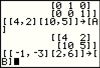Figure 40	Earlier we saw that multiplication of matrices is not, in general, commutative. Now we look at another seemingly strange behavior of matrices. We start out defining two new matrices and storing them in [A] and [B]. We should note that there is not even a single entry in either matrix that is 0.
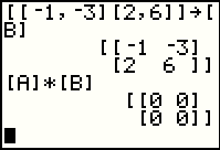Figure 41	Then we multiply the two matrices, [A] * [B], only to find that the product of these two non-zero matrices is the zero matrix. This is behavior that is quite different from that of numbers where we know that if the product of two numbers is zero that at least one of the two numbers must have been zero.
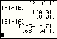Figure 42	Adding some interest to this turn of events, in Figure 42 we look at [B] * [A] only to find out that it is not the zero matrix!
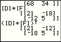Figure 43	Figure 43 returns to a discussion of matrix transposition from an earlier web page. Here we note first the matrix product [D] * [F], and then the value of that transposed, namely, ( [D] * [F] T. The second matrix is exactly what we would expect for a transposition.
Figure 44	Figure 44 first presents ( [F]T ) * ( [D]T ) which produces the same value as did ( [D] * [F] T. Thus we note that when we take the transposition of a product of matrices it is equal to the reversed product of the transposition of the two matrices. To give further evidence of this, look at Figure 44 to see the result of not reversing the order of the two matrices. We see that ( [D]T ) * ( [F]T ) not only does not produce the same values, it does not even produce a matrix of the same size!