In order to tie comments to specific locations in the book, I have used the available page ruler sheet to
identify lines in the text. A copy of that page ruler sheet can be printed from
The Index Sheet.
Chapter 2: Systems of Linear Equations and Matrices |
| 2.1 Systems of Two Equations in Two Unknowns |
| Page | Line # | Notes |
| 126 | 39 |
The text states that it is impossible to find the solution graphically. Of course, we could do it graphically on the
calculator and come so close that we could guess the solution.
Figure 1  |
First we enter the two equations from example 2 on page 126
|
Figure 2  |
Then we verify the WINDOW setting. This is the standard setting.
|
Figure 3  |
Then we move to the GRAPH screen.This looks much as does Figure 2 in the book.
|
Figure 4 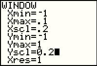 |
To approcimate Figure 3 in the book we change the WINDOW settings.
|
Figure 5  |
Return to the GRAPH screen.
To have the calculator solve this for us graphically, we move to the next screen by
pressing the   keys. keys.
|
Figure 6  |
Figure 6 shows the options for on the CALC screen. The option that we want
is 5:intersect which we select by pressing the  key. key.
|
Figure 7 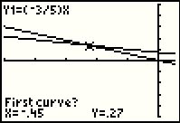 |
The calculator responds by suggesting a point on the first function. Unfortunately,
due to the settings of the WINDOW screen,
the point being suggested is right near the point of intersection and we cannot
really see which line holds the cursor. We move the
cursor tot he left a number of steps
to get to Figure 8.
|
Figure 8  |
Finally, on Figure 8, we see which line holds the cursor. The calculator is asking if this is the first curve.
to say yes, we press the  key and move to Figure 9. key and move to Figure 9.
|
Figure 9 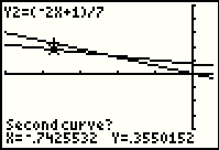 |
In Figure 9 we can see that our action if FIgure 8 left a marker on the first curve and that the calculator
has moved the cursor to the second curve to ask if it is OK to use this one as the second curve.
Again, we can press the  key to accept that offer. [This process seems absurd when only two
functions are being graphed. However, it may be the case that we have many functins on the graph. In that case we need to tell the
calculator which two functions to use. In that case the process makes sense.] key to accept that offer. [This process seems absurd when only two
functions are being graphed. However, it may be the case that we have many functins on the graph. In that case we need to tell the
calculator which two functions to use. In that case the process makes sense.]
|
Figure 10  |
Now the calculator has marked both fuunctions and it is asking for a guess, a location where it (the calculator)
can start its search for a point of intersection. In Figure 10 we have moved the cursor closer to the point of intersection. Then we press
the  key to start the calcualtor working. key to start the calcualtor working.
|
Figure 11 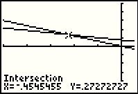 |
Figure 11 shows the result. The calculator has the x value of the solution at
-.4545455 which we recognize as probably a repeating decimal -0.454545454545....
The y value at the intersection is given as .27272727 which again implies 0.272727272727...
We could take those values and convert them to fractions to get (-5/11,3/11). Steps to do that are shown in Figure 12.
|
Figure 12  |
Figure 12 shows the conversion of 0.4545454545454545 to the fracton 5/11. This works because we have entered so many digits, more than the calcualtor really holds.
The same is true for 0.2727272727272727 as it is converted to 3/11.
|
|
| 138 | 37 |
Not that we use it all that often, but the term Inconsistent means that there is no solution
for the system of equations. This is an important concept.
|
| 129 | 19 |
The same can be said for the terms Redundant or Dependent describing situations where there are
infinitely many solutions. Because we have repeated an equation, possibly in a different form but just a repeat of
another equation, we really have one equation in two unkowns. Our ideal is to have two unique equations in two unkowns.
When we expand our systems to three unknowns we will want three unique equations, and so on.
|
| 2.2 Using Matrices to Solve Systems of Equations |
| Page | Line # | Notes |
| 137 | 30 |
Although the expansion to more unkowns gets messy quickly, it is important to note that
whereas two variables can be represented as coordinate axes on a plane and an equation of the
form Ax + By = C represents a line in that plane, three variables can be represented as space
(3-dimensions) marked off by a three-way coordinate axes system (length, width, height) and an
equation of the form Ax + By + Cz = =D represents a plane in that space.
|
| 139 | 37 |
There is a subtle switch here. Before the text just talked about multiplying a row by a non-zero constant or adding two
rows to get a new one. Now, in the Elementary Row Operations,
the book talks about replacing a row by the product of a non-zero constant and
the old contents of that row, or replacing a row by
the probuct of some non-zero number times the old contents of the row plus or minus some constant times another row.
|
| 139 | 37 |
The first note off to the side, the one marked as * NOTE,
deserves a bit more attention. We will actually follow
the "Some mathematicians insist that a=1 in and operation of Type 2."
We will do this because that is what our calculator will insist on doing. The command for this elementary row
operation is: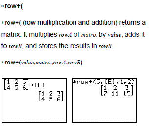
|
| 140 | 36 |
I find the book explanation of the Gauss-Jordan reduction to be too hard to follow, mainly because we do not know where we are going.
I will try to generate a web page with an alternate explanation and description, but it may take a bit to do that.
|
| 146 | 14 |
The example of an Inconsistent System is important in that you need to see that the
matrix ends up with an impossible row, one with all zero values except for the last item.
|
| 146 | 37 |
The example of infinitely many solutions is important in that you need to see that you end up with a row
of all zero values. That is similar to but different than the Inconsistent example given above it.
|
| | |
The web page Elementary Row Operations of the TI-83
goes through the steps to use the elementary row operations on the TI-83 to
take a matrix and put it through the Gauss-Jordan method. Please note that
the page assumes that you know how to create a matrix on the calculator. To help in that
the page does point you to the first 36 Figures of another page. If you are not comfortable using the
elementary row operations, it is worth reviewing these pages.
|
| 2.3. Applications of Systems of Linear Equations |
| Page | Line # | Notes |
| | |
No comment
|


 key.
key.


 key and move to Figure 9.

 key to accept that offer. [This process seems absurd when only two
functions are being graphed. However, it may be the case that we have many functins on the graph. In that case we need to tell the
calculator which two functions to use. In that case the process makes sense.]

 key to start the calcualtor working.


 keys.
keys.