More Linear Regression
Return to Topics page
Here is another typical textbook linear regression problem.
Table 1 gives 30 pairs of values, an X value and a Y value
in each pair.
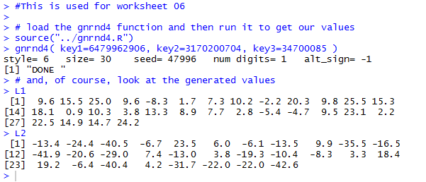
Thus, the first pair of values is the point (9.6,–13.4)
and the second pair is the point
(15.5,–24.4) and so on.
We will follow the usual procedure for doing our work on the USB drive.
In particular, we have
- inserted our USB drive,
- created a directory called
worksheet06
on that drive
- have copied
model.R from our root folder into
our new folder,
- have renamed that new copy of the file to the name
ws06.R, and
- have double clicked on that file to open RStudio.
The result should be a window pretty much identical to the one shown in Figure 1.
{Recall that the images shown here may have been reduced
to make a printed version of this page a bit shorter than
it woud otherwise appear.
In most cases your browser should allow you to right click on an image and then
select the option to View Image in order to see the image in its
original form.}
Figure 1
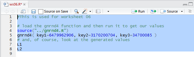
Our next step is to generate and verify the data that
we were given in Table 1.
Figure 2
The Console, in Figure 3,
shows the result of running the commands given in Figure 2.
Figure 3
Next we will get a quick plot of the points.
Figure 4

There is not much to see in the Console.
Figure 5

But the Plot pane, in Figure 6, shows the
scatter plot of the data.
Figure 6
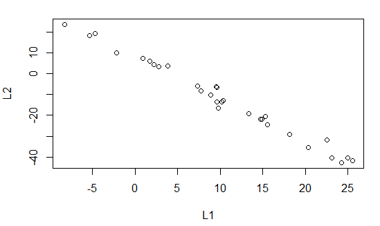
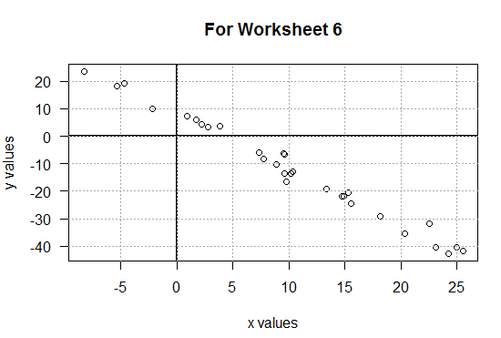
That plot certainly suggests a strong linear relation
between the values in L1 and the "paired"
values in L2.
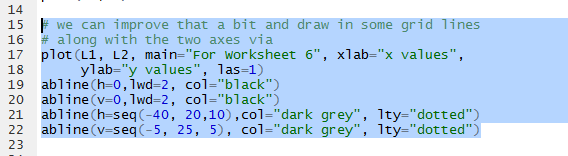
However, before we look at that relationship, we
can draw the graph again but this time clean it up a bit with a few
more commands. Those are shown, in the Editor pane in Figure 7.
Figure 7
Running those commands produces the much nicer looking
plot shown in Figure 8.
Figure 8
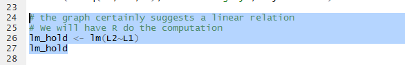
Then we can look at the linear model of the relationship by using the function
lm(L2~L1) shown in Figure 9.
Figure 9
Running those commands produces the rudimentary output shown in
the Console view in Figure 10.
Figure 10
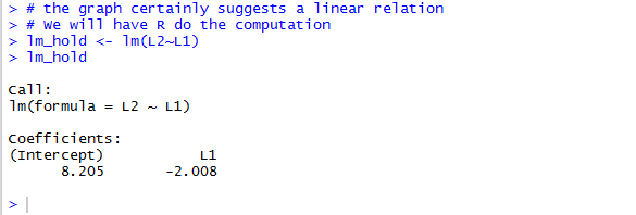
The information in Figure 10 is enough for us to fomulate the
linear regression equation
y = 8.205 + (-2.008)x
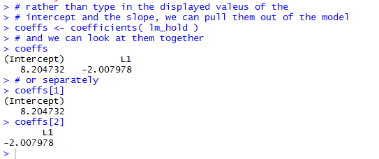
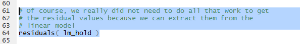
We have storeed the linear model in the variable lm_hold.
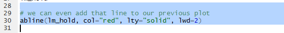
Therefore, the command shown in Figure 11, when run,
will produce the linear regression line in red on our graph.
Figure 11
Of course, this does not produce much at all in the Console pane.
Figure 12

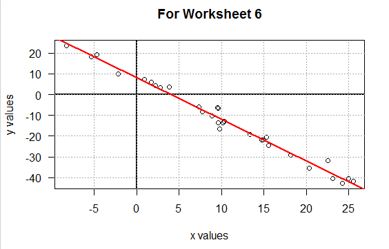
But the graph, in the Plot pane, now shows that line.
Figure 13
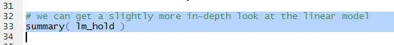
Where Figure 10 showed only the most essential information about our
linear model, we can formulate the command summary(lm_hold)
to give us more information about the model.
Figure 14
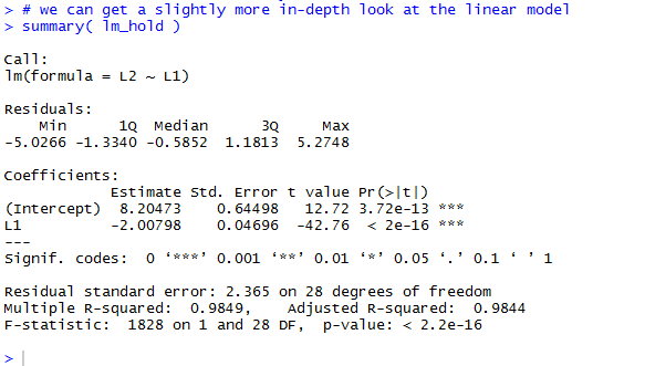
The result of running that command is shown in Figure 15.
Here we get information on the residual values,
more information about each of the two Coefficients,
and even more data that includes
the value for r2, namely 0.9849.
Figure 15
The commands shown in Figure 17 allow us to look at an, eventually use, the coefficient
values without retyping them.
Figure 16
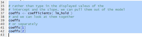
Looking at Figure 17 and refering back to Figures 10 and 15,
we can see that we have the coefficient values in variables
that we can use.
Figure 17
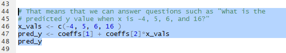
One such use would be to find the values that we would expect,
the values that the equation ould predict for given values of x.
That is, we can answer the question "What are the exected values from
our model if x has the value -4? Or if x has the value
5, or 6, or 16?"
To do this we can put those x-values into a variable,
in this example it is called x_vals, and then
we can evaluate our linear regression equation for each of those values.
Figure 18 holds the commands to do this.
Figure 18
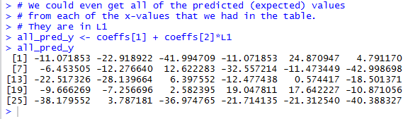
Running those commands produces the output shown in Figure 19.
Figure 19

The interpretation of those values is
- if x = -4, then the regression equation expects y to be 16.236643,
- if x = 5, then the regression equation expects y to be -1.835156,
- if x = 6, then the regression equation expects y to be -3.843134, and
- if x = 16, then the regression equation expects y to be -23.922911.
It is interesting to note that raising the x value by 1 changes the
y value by the exat amount of the slope, the second coefficient.
This is exactly what we would expect from the equation
y = 8.205 + (-2.008)x
Also, please note that the four values that we used for x, namely, -4, 5, 6, and
16, are all within the range of the x-values; they go from -8.3 to 25.5. Therefore,
the four examples are all interpolations. There is nothing stopping us from
using the regression equation to find the expeted value when x is outside of that
range, say for x=-12 or x=30, but those would be
extrapolations, and as such they are muh more suspect.
Rather than just find the four points given above, we could use the same tehnique
to find the expected values for all of the original x-values.
The commands to do this are given in Figure 20.
Figure 20
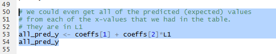
Figure 21 show the results of running those commands.
Figure 21
But, since we have the observed values, the y-values in
Table 1, and
we now have the
expected values, we can find the residual values by
finding the observed - expeted values via the
command L2-all_pred_y, as shown in Figure 22.
Figure 22
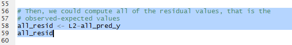
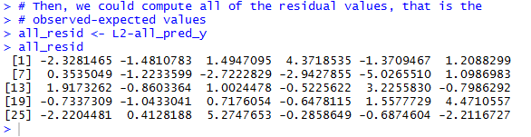
Figure 23 gives the Console view of running those commands.
Figure 23
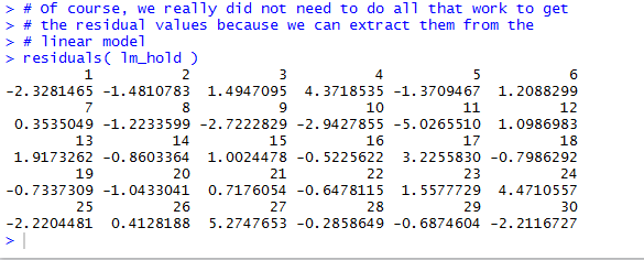
Of course, we did not have to do any of that computation. The
linear model, lm_hold, actually contains the residuals.
We use the command
residuas(lm_hold) to extract those values from
the model.
See Figure 24.
Figure 24
The values are seen in Figure 25. There each value is shown with its
sequential number, but the residual values displayed are the same as those that
we computed and saw in Figure 23.
Figure 25
The reason that we want the residual values is that we want to look at the
plot of the L1 values agains the residual values.
The command is shown in Figure 26.
Figure 26
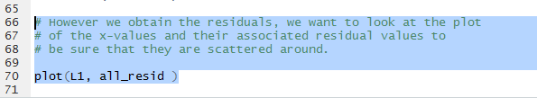
The desired plot is shown in Figure 27. The
important part of this is that we should find the plotted points
spread out, without a pattern, aross the graph. In this case that is true.
If it were not true then we would have some concerns about
the regression equation. [See worksheet06a
for an example where the residuals
do not scatter all over the place.]
Figure 27
Recall that in Figure 15 we saw that the r2
value was 0.9849, indicating that the linear model explains about 98.5% of the
variability of the data. This is actually the square of the correlation coefficient
that we call r. To compute r directly
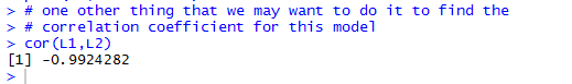
we use the cor(L1,L2) command shown in Figure 28.
Figure 28
The result, shown in Figure 29, gives r= = -0.9924282.
Note that the value is negative, which we expect sine the slope of
our linear regression line is negative.
Figure 29
That is enough for this example. We note that we have yet to save our
ws06.R file, since its name is in red letters (Figure 30).
Figure 30

We click on the  icon to save the file,
turning the file name use black letters (Figure 31).
icon to save the file,
turning the file name use black letters (Figure 31).
Figure 31

In the Console we give the command q(),
press ENTER, then respond to the prompt with y (Figure 32).
Figure 32

Then press ENTER to terminate the RStudio session. Figure 33
shows the then current status of our
directory (folder), showing our ws06.R file along with, since this was done on a Windows
machine, the two hidden files .RData and .Rhistory.
Figure 33

Here is a listing of the complete contents of the descriptive.R
file:
#This is used for worksheet 06

# load the gnrnd4 function and then run it to get our values
source("../gnrnd4.R")
gnrnd4( key1=6479962906, key2=3170200704, key3=34700085 )
# and, of course, look at the generated values
L1
L2


# the values look good.
# generate a quick and dirty scatter plot
plot(L1,L2)

# we can improve that a bit and draw in some grid lines
# along with the two axes via
plot(L1, L2, main="For Worksheet 6", xlab="x values",
     ylab="y values", las=1)
abline(h=0,lwd=2, col="black")
abline(v=0,lwd=2, col="black")
abline(h=seq(-40, 20,10),col="dark grey", lty="dotted")
abline(v=seq(-5, 25, 5), col="dark grey", lty="dotted")

# the graph certainly suggests a linear relation
# We will have R do the computation
lm_hold <- lm(L2~L1)
lm_hold

# we can even add that line to our previous plot
abline(lm_hold, col="red", lty="solid", lwd=2)

# we can get a slightly more in-depth look at the linear model
summary( lm_hold )

# rather than type in the displayed valeus of the
# intercept and the slope, we can pull them out of the model
coeffs <- coefficients( lm_hold )
# and we can look at them together
coeffs
# or separately
coeffs[1]
coeffs[2]

# That means that we can answer questions such as "What is the
# predicted y value when x is -4, 5, 6, and 16?"
x_vals <- c(-4, 5, 6, 16 )
pred_y <- coeffs[1] + coeffs[2]*x_vals
pred_y

# We could even get all of the predicted (expected) values
# from each of the x-values that we had in the table.
# They are in L1
all_pred_y <- coeffs[1] + coeffs[2]*L1
all_pred_y

# Then, we could compute all of the residual values, that is the
# observed-expected values
all_resid <- L2-all_pred_y
all_resid

# Of course, we really did not need to do all that work to get
# the residual values because we can extract them from the
# linear model
residuals( lm_hold )

# However we obtain the residuals, we want to look at the plot
# of the x-values and their associated residual values to
# be sure that they are scattered around.

plot(L1, all_resid )

# one other thing that we may want to do it to find the
# correlation coefficient for this model
cor(L1,L2)
Return to Topics page
©Roger M. Palay
Saline, MI 48176 February, 2017