Using the distribution of the sample mean
Return to Topics page
The previous web page, The Sample Mean,
was meant to convince us that for a given population with mean μ
and standard deviation σ if we take samples of size n (with replacement)
then the distribution of the sample means will be normal with mean μ
and standard deviation σ/sqrt(n), especially if n is 30 or larger or if
the original population had a normal distribution.
The consequence of this is that we can answer some more challenging questions.
We will start with a old problem that we know how to do.
If we have an approximately normal
population with mean 23.4 and standard deviation 6.1,
then we can compute the probability that a single random sample of that population
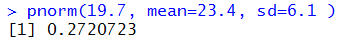
is less than 19.7, i.e., P(X<19.7). In R we use the
statement pnorm(19.7, mean=23.4, sd=6.1 ) to find that the
probability is 0.272. We can see this in Figure 1.
Figure 1
This result is what we expect. After all, if the population mean is
23.4 and the standard deviation is 6.1 then for a normal
population we expect to have about 16% of the values be lower than
23.4 – 6.1 or 17.3.
It makes perfectly good sense then to find
27.2% of the values to be less than 19.7.
Now, if we have a sample of size 22 of that population,
we can ask what is the probability that the sample mean will be
less than 19.7? Because we are asking about the
sample mean we need to use the fact that the
sample means will be N(23.4,6.1/sqrt(22)).
But the square root of 22 is about 4.69
and 6.1/sqrt(22) is about 1.3.
One standard deviation below the mean is about
23.4 – 1.3 or 22.1.
Our value, 19.7 is way lower than that.
In fact, 19.7 is about 2.845 standard deviations
below the mean. We recall that only about 0.135% of the
values are lower than 3 standard deviations below the mean.
We should expect that the probability of getting a sample mean less
than 19.7 (i.e., a value that is 2.845 standard deviations
below the mean) will be just slightly larger than that 0.135%.
The R statement to find this is
pnorm(19.7, mean=23.4, sd=6.1/sqrt(22) )
as shown in Figure 2.
Figure 2

The result, 0.00222, or 0.222%, is right where we expected it would be.
If we have a population, heavily skewed to the right, but with mean 137.2
and standard deviation 12.7, we might be interested in finding the probability that
a random item from that population is greater than 140? Unfortunately,
because we do not know the distribution of the values in the population, we cannot answer
that question. However, if we take a sample of size 43 (a sample well larger than 30)
then we can ask, and answer, "What is the probability that the mean of
the 43-item sample will be greater than 140?"
We can do this because we know that the sample mean for such a large
sample will be normal with mean=137.2 and
standard deviation=12.7/sqrt(43).
Therefore, in R, we can use the command
pnorm(140,mean=137.2,sd=12.7/sqrt(43),lower.tail=FALSE)
as shown in Figure 3.
Figure 3

The answer, 0.0741, fits well with our understanding of the
normal distribution in that 140 is about 1.45
standard deviations above the mean. But remember, that is
standard deviations of the sample means (i.e., 12.7/sqrt(43))
not standard deviations of the population.
If we have a bimodal population with mean=4.21 and
standard deviation=17.3 we would have no way of answering
the question "What is the probability of taking a sample and
having its value no more than 4 away from the mean?"
However, even though the population is bimodal we know that the distribution of the
sample means will be normal with mean=4.21 and
standard deviation=17.3/sqrt(n) where n is the size of the samples.
Therefore, we can ask and answer the question
"What is the probability a sample of size 53 will have its sample mean
no more than 4 away from the mean?"
That is the same as P(0.21≤xbar≤8.21).
We can compute that as
P(xbar≤8.21) – P(xbar≤0.21),
or in the R language
we could do
samp_sd <- 17.3/sqrt(53)
samp_sd  #just to see the value
pnorm(8.21, mean=4.21, sd=samp_sd) -
   pnorm( 0.21, 4.21, samp_sd)
This is shown in Figure 4.
Figure 4
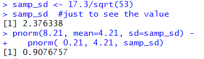
We see that the probability of being between those values is about 0.908.
Or, how about this problem. We are making cereal and packaging it into
boxes that say they hold 24 ounces of the product. We know that the machine that fills the boxes
operates with a mean box weight of 24 ounces and a standard deviation of the
box weight at about 0.2 ounces. In order to not run afoul of the law,
we sure do not want boxes that weigh less than 23.9 ounces.
In order to not give way too much we sure do not want boxes that hold more than 25 ounces.
What is the probability that a sample box will weigh
less than 23.9 ounces or more than 25 ounces?
Offhand we cannot answer this because we do not know the distribution of the weight of the boxes.
If someone comes along and says that the distribution is normal
then we could find P( x≤23.9 or x ≥25 )
by the R commands
# find prob x < 23.9 or x > 25, assuming a
# normal distribution

pnorm( 23.9, 24, 0.2) +
     pnorm( 25, 24, 0.2, lower.tail = FALSE)
shown in Figure 5.
Figure 5
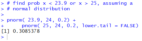
That result means the almost 31% of the boxes of cereal will be outside of the
desired range. That is not good.
On the other hand, we do not ship individual boxes to customers, we send pallets of
boxes to customers. There are 48 boxes in each pallet.
The process of assembling a pallet, as it turns out in our special case,
really mimics taking a random sample of the boxes. That is, we do not take sequentially filled boxes
to make up a pallet. There is no predicting if a particular box will or
will not make it into the next pallet. So, we could consider the boxes
in the pallet to be a random sample of 48 of our cereal boxes.
Furthermore, we know that
our customers, the stores that buy our cereal, are really concerned about the average
weight of the boxes in the pallet, not about the weight of individual boxes.
So, we ask a new question, "What is the probability that the mean weight of
boxes in a pallet is less than 23.9 ounces or more than 25 ounces?"
To answer this we need to use the standard deviation of the sample
mean, in this case that will be 0.2/sqrt(48).
We are looking for
P( xbar≤23.9 or xbar ≥25 )
which we can express in R by
#
# then find prob  xbar < 23.9 or xbar > 25 for
#     a sample of size 48
samp_sd <- 0.2/sqrt(48)
pnorm( 23.9, 24, samp_sd) +
   pnorm( 25, 24, samp_sd, lower.tail = FALSE)
Figure 6 shows the R response to those commands.
Figure 6
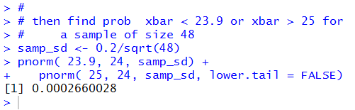
From this we see that we expect that fewer than 3 out
of every 10,000 pallets will be in the undesirable range.
This is good.
Return to Topics page
©Roger M. Palay
Saline, MI 48176 October, 2016