Measures of Dispersion

Return to Descriptive Measures

This page gives a more detailed discussion of the range, quartiles , and standard deviation.

Range

Of the three measures presented here, the range is the most straightforward. It is simply the lowest and highest value in the data collection. For example, although it might be hard to just see, the lowest and highest value in the numbers shown in Table 1 (those values can be created by

This does leave us with the question of finding these range values in R. To demonstrate this we need a table that has fixed values, such as Table 2, whose values are created by

Here are the commands that we will use to generate the list of values and then to find the minimum value and the maximum value:

# We want to use gnrnd4 so we need to load it
#      into our environment
source("../gnrnd4.R")
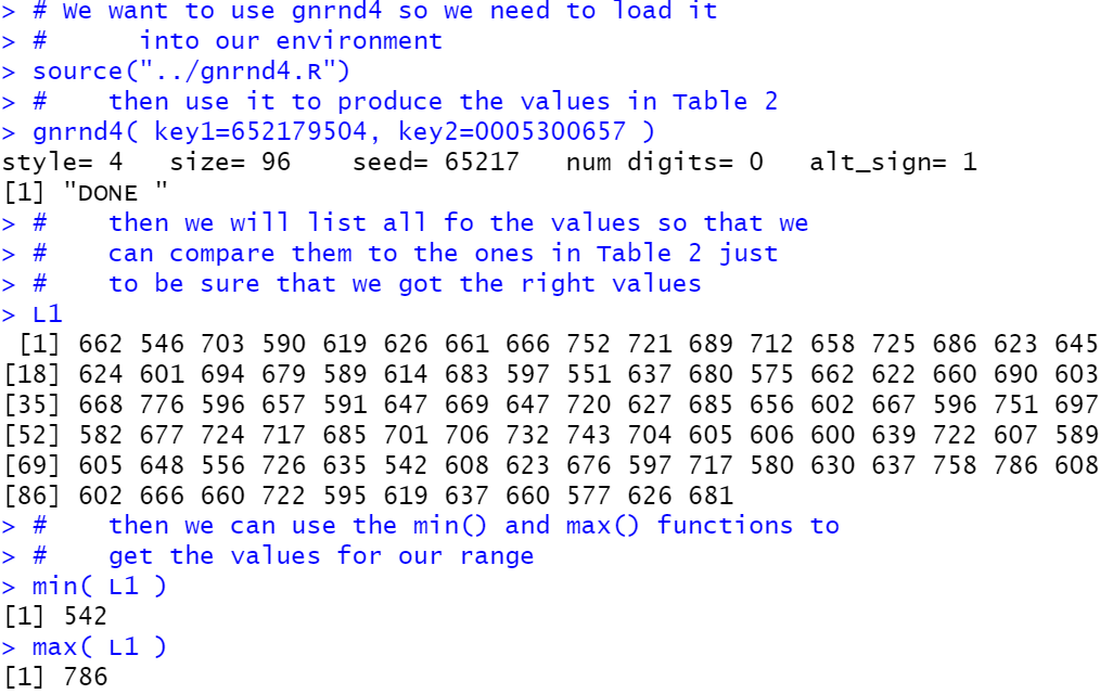
#    then use it to produce the values in Table 2
gnrnd4( key1=652179504, key2=0005300657 )
#    then we will list all fo the values so that we
#    can compare them to the ones in Table 2 just
#    to be sure that we got the right values
L1
#    then we can use the min() and max() functions to 
#    get the values for our range
min( L1 )
max( L1 )

Figure 1 shows using those commands to generate the data in R, displaying the data just to be sure that we have it correct, and then finding the minimum and maximum values, that is, the range values. Figure 1

In R we can use the min() function to find the minimum value in the collection and the max() function to find the maximum value in the collection. We can get both of these same values via a different R function, namely the summary() function, but we will present that in the next section.

Quartiles

Recall that in the discussion of measures of central tendency we looked at the median value. The median is the value such that half the data values are less than or equal to the median and half are greater than the median. We do not care how much less or how much greater values are; we just want to know the middle value.

Quartiles extend that concept to dividing the data into four "equal sized" pieces. For the quartiles we want three values, we call them Q₁, Q₂, and Q₃, such that, as close as we can make it, ¼ of the data points are less than or equal to Q₁, ¼ of the data points are between Q₁ and Q₂, ¼ of the data points are between Q₂ and Q₃, and ¼ of the data points are greater than or equal to Q₃. You should note that as a consequence of this, Q₂, which has 50% of the values below and above it, is really just the median.

One can look at this as saying that Q₁ is really the median of the lower half of the points, while Q₃ is really the median of the upper half of the points. This works, in a general sense, and it should make it easier to understand the concept of the quartiles.

There is a problem once we get to the details of finding the quartiles and that problem is really an extension of the problem we had with the median. Recall, that for an odd number of values the median is an actual data point. However, for an even number of values, we needed to make the median equal to the mean of the two middle data points. We calculate Q₂ exactly the same way. However, it is not clear how to calculate either Q₁, or Q₃. To begin, if there is an odd number of values then Q₂ is one of them. Should our calculation for Q₁ include that value or not. The same is true for Q₃. On the other hand, if there is an even number of values then Q₂ is not one of the data points (though it could be equal to two or more of them). For an even number of data values should the points used to find Q₂ be included or excluded in finding, let us say, the median of the lower half of the values, Q₁? And so on.

In the end, there is not a single, uniformly agreed upon, rule for computing the quartiles, Q₁ and Q₃. If you use a TI-83/84 calculator to find the quartiles you will get an answer, but it may not be the same answer that you get if you ask Minitab to do the same computation, or if you ask Excel or R to do the calculation. We can return to the data in Table 2 for a more specific look at the quartiles. of that data.

One thing that we can do is to sort the 96 values in that table. Table 2-sorted does this along with highlighting the 48^th and 49^th items. Because there are an even number of items, 96, in our list, the median is the mean of those two middle items in the sorted list. Therefore, Q₂'s value is Q₂=(648+656)/2=652.

Sorting the data would certainly allow us to figure out the values of Q₁ and Q₃ by inspection (assuming that we had an agreement about how to actually find the points). On the other hand, if we put the same collection of values into a TI-83/84 calculator and then issue the 1-Var Stat command, the calculator responds with Figure TI

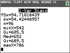
which clearly shows the value of Q₁ as 605.5 and the value of Q₃ as 689.5. (It is somewhat reassuring to have the TI-83/84 also show us the same values for the minimum, 542, the maximum, 786, and the median, 652, that we knew to be correct.]

Alternatively, in our R session we could ask R to sort the values just so that we can compare them to the values in Table 2-sorted. Then, via the summary() function, we could get the output shown at the bottom of Figure 2. First, here are the commands that we will use

#    We want to see the sorted list of values
sort( L1 )
#    We use the summary() function to get the Q1 and Q3 values
summary( L1 )

Figure 2

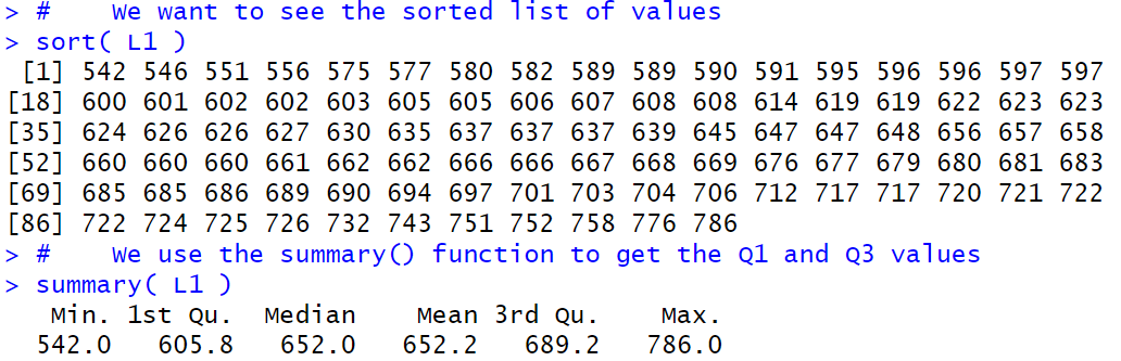
In Figure 2 we see that R gives us the same values for the minimum, median, and maximum. However, R shows the value 605.8 for Q₁ and the value 689.2 for Q₃. Different values than we found on the TI calculator, though not much different.

As was the case in our discussion of the median, this difference often disappears in larger data collections where there a many repetitions of values in the collection. In those situations, the "averaging" that shows up in some cases for finding quartile points between data points ends up being the average of identical values.

The bottom line for us, in this course, is that we will use the quartile values determined by the summary() command in R. However, we should be a bit concerned because of the few decimal digits that are shown in the output of the summary() command. We notice that the mean given by the summary() function is 652.2. However, as we see in Figure 2a, R computes and displays the mean with more significant digits as 652.2188.

Figure 2a

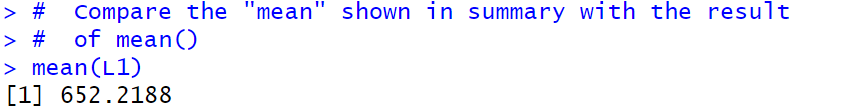
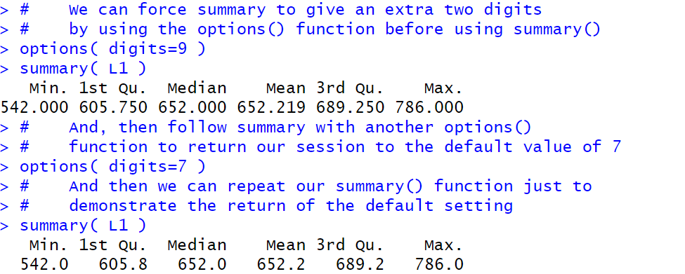
Clearly, the value shown in Figure 2 is a rounded one. Therefore, we must assume that the values shown back in Figure 2 for Q₁ and Q₃ are also rounded. The question becomes, "How do we get summary() to show more significant digits of the computed values?" The answer to that is to insert the command options(digits=9) before we use the summary() command. This is shown in Figure 2b, along with a subsequent options(digits=7) command that will reset R to the defaut number of digits.

Here are the commands we will use to generate Figure 2b:

#    We can force summary to give an extra two digits
#    by using the options() function before using summary()
options( digits=9 )
summary( L1 )
#    And, then follow summary with another options()
#    function to return our session to the default value of 7
options( digits=7 )
#    And then we can repeat our summary() function just to 
#    demonstrate the return of the default setting
summary( L1 )

Figure 2b

With the extra digits displayed we see that Q₁ = 605.75, not 605.8, and Q₃ = 689.25, not 689.2. In case you were counting, the value specified in the options() command gives R an "idea" of the space to allocate, not a specific hard and fast rule.

It is a little bit of a pain to keep changing the number of digits to be displayed just so that we can get decent values for Q₁ and Q₃. Here are two alternatives. First we can use the quantile() function as an alternative way to get Q₁ and Q₃. We will use the command

#    Let us look at two alternative ways fo find the quartiles.
#    First, R has a command, quantile(), that we can use to find
#    the 25th and 75th percentiles, which are the first and 
#    third quartiles.
quantile( L1, c( 0.25, 0.75 ))
#    Using the quantile() function has the advantage of showing
#    more significant digits than we had using the summary()
#    function.

Figure 2c

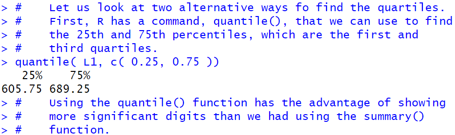
In this case we can see that the quantile() function shows more digits. In fact it would show 7 if it needed that many.

A second approach is to use the long_summary() function. This is a function that you should have in your directory of extra functions. We can use the following commands to load and run long_summary().

#    As noted in the text, there are different acceptable ways
#    to compute Q1 and Q3.  R uses one method, the TI-83/84 
#    calculators use a different method and therefore, at times,
#    get Q1 and Q3 values that are different than what we 
#    get with R.
#    It would be nice to see those alternative values.  The 
#    function long_summary() will do this.  However, we need to
#    load long_summary() into our environment before we
#    can use it.
source("../long_summary.R")
#    Now that it is loaded we can use it
long_summary( L1 )

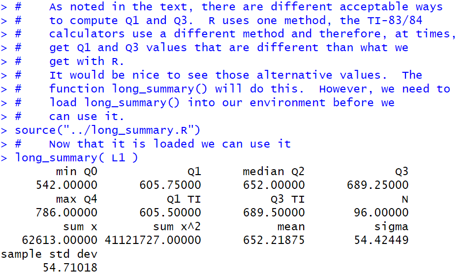
This will produce the following: Figure 2d

We see that the output from Q₁ includes everything that we got from the summary() command along with maany more values, including the Q₁ and Q₃ values that we would get if we had a TI-83/84 calculator do this work for us. Furthermore, the long_summary() function produces values with the full 7 digits of display (set by the default value that we restored way back in Figure 2b.

Standard Deviation

On the Descriptive Measures page we saw that the definition of the standard deviation for `n` data values, `x_1, x_2, x_3,...,x_(n-1),x_n` was given by `sigma = sqrt((sum_(i=1)^n ( x_i-mu)^2)/n)` which is a nice mathematical definition. Once we have access to software such as R we have less need for trying to find an equivalent formula that might be easier to compute. However, since this is to some extent a math class, we should look at developing a different formula. Rather than put all that ugly math here I have created a web page to show the development of an alternative formula, namely,

, for computing the standard deviation.

Of course, if we really wanted to, we could go through all of the steps needed to compute, in R, the standard deviation by following either of the two formulae. Such steps are really not worth it since R has a command, sd(), that would seem to do the computation for us. However, let us take just a few minutes to go through the process of evaluating each formula for our data just to see that they not only give us the same answer but also that the built-in R function produces that same value. We will use the data in Table 2 for this.

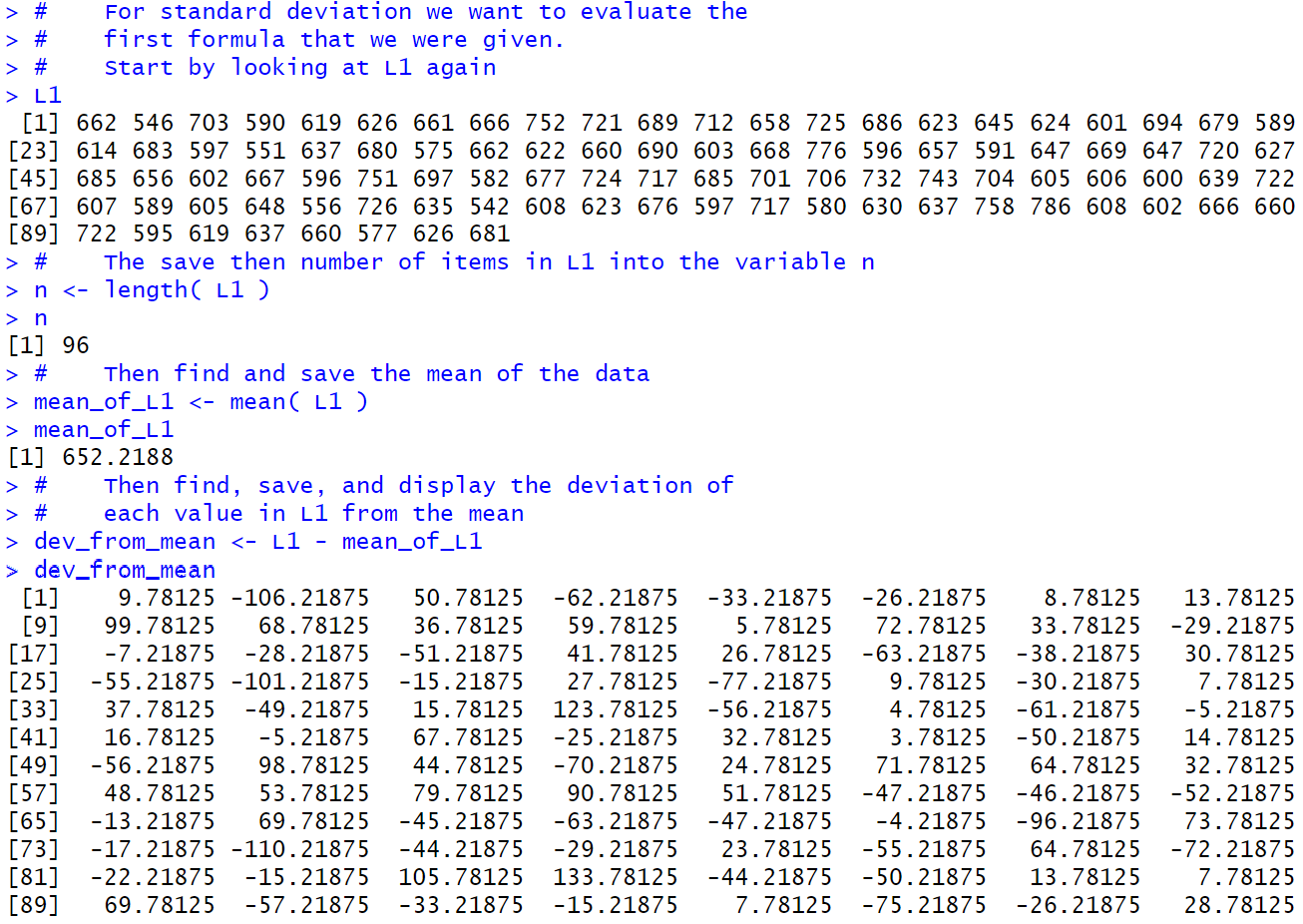
First, let us evaluate `sigma = sqrt((sum_(i=1)^n ( x_i-mu)^2)/n)`. The steps to do this, or at least to do the start of this, are shown in Figure 3. Note that in most cases I have chosen to show the computed values immediately after the computation, but such a display is just meant to help in confirming what is going on. It is not at all required for the actual determination of the standard deviation.

We start by showing the contents of L1. After that we put the length of L1 into the variable n. Once we have that we can compute the mean of the data which we store in mean_of_L1. Now that we have the mean we can compute the deviation from the mean for each value in L1. We store all 95 of these values in dev_from_mean and the display of those values, when compared to the values in L1 should convince you that that is exactly what happened.

Here are the commands we will use:

#    For standard deviation we want to evaluate the
#    first formula that we were given.
#    Start by looking at L1 again
L1
#    The save then number of items in L1 into the variable n
n <- length( L1 )
n    
#    Then find and save the mean of the data
mean_of_L1 <- mean( L1 )
mean_of_L1
#    Then find, save, and display the deviation of
#    each value in L1 from the mean
dev_from_mean <- L1 - mean_of_L1
dev_from_mean

Figure 3

Then we can continue the process in Figure 4. There our first step is to get the square of each of those deviations from the mean. We put those 95 values into sq_of_dev, and again display the results just for our own benefit. Just below halfway in Figure 4 we find the sum of the squared deviations from the mean and store that in sum_sq_dev. We move from there to find the mean squared deviations from the mean and store that into mean_sum_sq_dev. Finally, we compute the root mean squared deviations from the mean and store this in root_mean_ssd. This is the standard deviation.

Here are the commands we will use:

#    Now find all the squares of those deviations
sq_of_dev <- dev_from_mean^2
sq_of_dev
#    the find, store, and display the sum of the squared deviations
sum_sq_dev <- sum( sq_of_dev )
sum_sq_dev
#    divide that sum by the number of items to get the mean
mean_sum_sq_dev <- sum_sq_dev / n
mean_sum_sq_dev
#    Finally, take the square root of that mean
root_mean_ssd <- sqrt( mean_sum_sq_dev )
root_mean_ssd

Figure 4

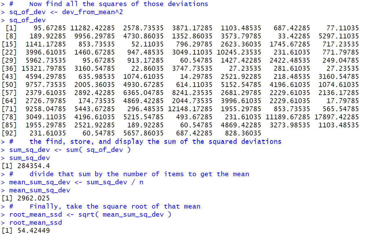
Thus, using the basic definition of standard deviation we get the value 54.42449.

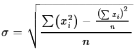
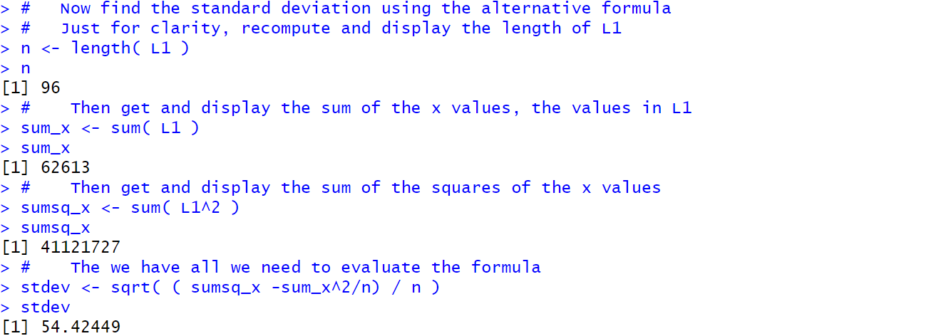
Let us do the computation using the alternative formula: `sigma = sqrt( ("sumsqx" - ("sumx")^2/n)/n)`. We start, in Figure 5, by restating the value of n. After that we get the sum of the values and store that in sum_x. Then we compute the sum of the squares of the values and store that in sumsq_x. At that point we are ready to just compute the standard deviation which turns out to be exactly the same value, 54.42449.

Here are the commands we will use:

#   Now find the standard deviation using the alternative formula
#   Just for clarity, recompute and display the length of L1
n <- length( L1 )
n
#    Then get and display the sum of the x values, the values in L1
sum_x <- sum( L1 )
sum_x
#    Then get and display the sum of the squares of the x values
sumsq_x <- sum( L1^2 )
sumsq_x
#    The we have all we need to evaluate the formula
stdev <- sqrt( ( sumsq_x -sum_x^2/n) / n )
stdev

Figure 5

It is somewhat comforting to see that we get the same result using either formula and that, as advertised, the second formula is easier to compute than is the first. You might also note that the output for the long_summary() function included the values for the sum of the values and the sum of the squared values.

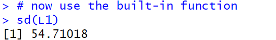
We now turn our attention to the R built-in function sd(), which looks like it should yield the standard deviation. At the top of Figure 6 we ask for sd(L1) and we get the answer 54.71018, which is close, but not the same as the two answers that we got before.

Figure 6

What is wrong? Where did we make a mistake?

The problem is that the sd() function in R computes the standard deviation for a sample and all of the work that we have done has been to find the sample deviation for a population. At this point in the course we have yet to talk about the difference between a sample and a population. It looks like we need to at least introduce that distinction here so that we can move forward. The standard deviation for a sample, usually called `s_x`, is given by the defining formula:

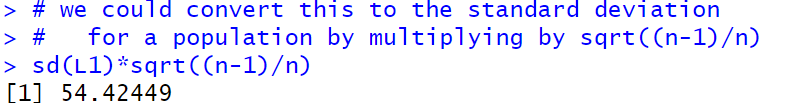
`s_x = sqrt((sum_(i=1)^n ( x_i-mu)^2)/(n-1))` We notice that the only difference between that formula and the defining formula for the standard deviation of a population `sigma = sqrt((sum_(i=1)^n ( x_i-mu)^2)/n)` is the denominator, for a sample we use n-1 whereas for a population we use n. Therefore, mathematically, if we have the value for `s_x` we can multiply it by `sqrt((n-1)/n)` and the result will be the value of `sigma`. We will attempt this in Figure 6.5. Figure 6.5

Relief! We got the same answer, 54.42449, that we computed above.

Of course, making that adjustment in R whenever we want to get the standard deviation of a population is not convenient at all. A better solution is for us to construct our own function that will take care of this for us. You have been given such a function, called pop_sd(), in the file called pop_sd.R. We can load that file into our environment via the source("../pop_sd.R") command as shown in Figure 7.

Figure 7

Now that the function is in the environment we can just go ahead and use it, as shown in Figure 8.

Figure 8

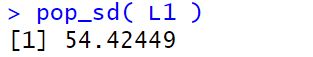
We get exactly the result that we expect.

Although this is not a programming course, a look at the function pop_sd() shows us that it is doing just what we would do by hand. It finds the length of the list of values and then takes the standard deviation for a sample, sd(), and multiplies it by the square root of (n-1)/n. Here is a listing of the lines of the function:

pop_sd<-function( input_list )
{ n <- length( input_list)
  sd( input_list )*sqrt((n-1)/n)
}

It is important to remember to use sd() to find the standard deviation of a sample and to use pop_sd() to find the standard deviation of a population (and remember that sd() is a built-in function, but pop_sd() must be loaded into your environment).

You should also note that the standard deviation of the data as a population and the standard deviation of the same data as a sample is given in the output of the long_summary() function, back in Figure 2d.

Here are all of the R statements used on this page:


# We want to use gnrnd4 so we need to load it
#      into our environment
source("../gnrnd4.R")
#    then use it to produce the values in Table 2
gnrnd4( key1=652179504, key2=0005300657 )
#    then we will list all fo the values so that we
#    can compare them to the ones in Table 2 just
#    to be sure that we got the right values
L1
#    then we can use the min() and max() functions to 
#    get the values for our range
min( L1 )
max( L1 )
#    We want to see the sorted list of values
sort( L1 )
#    We use the summary() function to get the Q1 and Q3 values
summary( L1 )
#  Compare the "mean" shown in summary with the result
#  of mean()
mean(L1)
#    We can force summary to give an extra two digits
#    by using the options() function before using summary()
options( digits=9 )
summary( L1 )
#    And, then follow summary with another options()
#    function to return our session to the default value of 7
options( digits=7 )
#    And then we can repeat our summary() function just to 
#    demonstrate the return of the default setting
summary( L1 )
#    Let us look at two alternative ways fo find the quartiles.
#    First, R has a command, quantile(), that we can use to find
#    the 25th and 75th percentiles, which are the first and 
#    third quartiles.
quantile( L1, c( 0.25, 0.75 ))
#    Using the quantile() function has the advantage of showing
#    more significant digits than we had using the summary()
#    function.

#    As noted in the text, there are different acceptable ways
#    to compute Q1 and Q3.  R uses one method, the TI-83/84 
#    calculators use a different method and therefore, at times,
#    get Q1 and Q3 values that are different than what we 
#    get with R.
#    It would be nice to see those alternative values.  The 
#    function long_summary() will do this.  However, we need to
#    load long_summary() into our environment before we 
#    can use it.
source("../long_summary.R")
#    Now that it is loaded we can use it
long_summary( L1 )

#    For standard deviation we want to evaluate the
#    first formula that we were given.
#    Start by looking at L1 again
L1
#    The save then number of items in L1 into the variable n
n <- length( L1 )
n    
#    Then find and save the mean of the data
mean_of_L1 <- mean( L1 )
mean_of_L1
#    Then find, save, and display the deviation of
#    each value in L1 from the mean
dev_from_mean <- L1 - mean_of_L1
dev_from_mean

#    Now find all the squares of those deviations
sq_of_dev <- dev_from_mean^2
sq_of_dev
#    the find, store, and display the sum of the squared deviations
sum_sq_dev <- sum( sq_of_dev )
sum_sq_dev
#    divide that sum by the number of items to get the mean
mean_sum_sq_dev <- sum_sq_dev / n
mean_sum_sq_dev
#    Finally, take the square root of that mean
root_mean_ssd <- sqrt( mean_sum_sq_dev )
root_mean_ssd

#   Now find the standard deviation using the alternative formula
#   Just for clarity, recompute and display the length of L1
n <- length( L1 )
n
#    Then get and display the sum of the x values, the values in L1
sum_x <- sum( L1 )
sum_x
#    Then get and display the sum of the squares of the x values
sumsq_x <- sum( L1^2 )
sumsq_x
#    The we have all we need to evaluate the formula
stdev <- sqrt( ( sumsq_x -sum_x^2/n) / n )
stdev

# now use the built-in function
sd(L1)

# we could convert this to the standard deviation
#   for a population by multiplying by sqrt((n-1)/n)
sd(L1)*sqrt((n-1)/n)

# or we could codify that in a new function
source("../pop_sd.R")
pop_sd( L1 )

Return to Descriptive Measures