| Figure 1 |
|
|
This page is based on the installation of RStudio
on a PC computer using the Firefox web browser.
The process took place on August 14, 2015.
The standard version of RStudio
at that time was 0.99.467.
Please understand that web pages change, software changes,
and installation systems change. Thus, what is recorded here,
although true at the moment of
recording, may have changed by the time you read this.
Also, as I hope is obvious, the images below have been annotated, in GREEN, to show you where you need to point and click. Just a few quick notes:
|
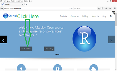
To install RStudio, we will go to the RStudio web site at the https://www.RStudio.com/ web site. This should open a page, the top of which should appear as shown in Figure 1.
| Figure 1 |
|
|
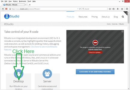
We will click on the "Download RStudio" button, as shown in Figure 1. Most likely, the result will be the screen shown in Figure 2. Your only clue as to the next step is to click on the "Desktop" version. That is the action suggested here. [However, if you just point the that same "Desktop" icon, you will see that it is just a link, https://www.RStudio.com/products/RStudio/#Desktop, to the same web page, just further down the page than we are in Figure 2. That is, you could just scroll down and get to the same place.]
| Figure 2 |
|
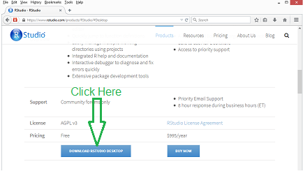
The result of your navigation should be the screen shown in Figure 3. You may need to scroll down to find the "DOWNLOAD RStudio DESKTOP" button. Then, click on that button.
| Figure 3 |
|
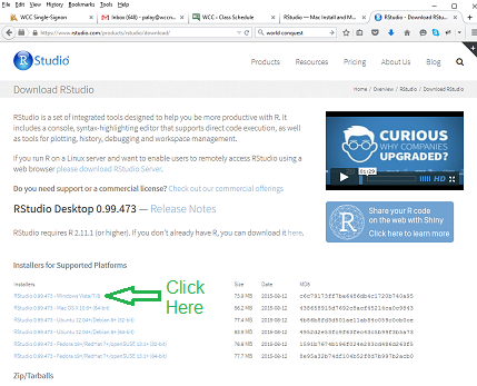
On this screen, the one shown in Figure 4, you finally get to make the choice of the version of RStudio to install. We, of course, want to select the "RStudio 0.99.467 – Windows Vista/7/8/10" option.
[Note that you could have just started at this page if you had used the URL https://www.RStudio.com/products/RStudio/download/ to start.]
| Figure 4 |
|
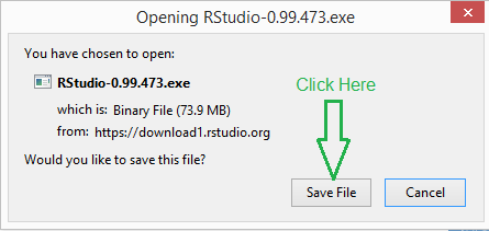
The computer responds with the screen shown in Figure 5. Our response is to just click on the "Save File" button.
| Figure 5 |
|
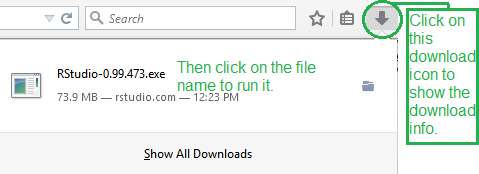
The particular browser used here, Firefox, did not have any special customization for placing downloaded files. Therefore, in this case, the downloaded or "saved" file will be in the default directory. We will not even concern ourselves with the location of the downloaded file, because, in Firefox, there is an icon in the tool bar to let us look at the recently downloaded files. Naturally, other browsers may behave in different fashions. Our next action is to "run" the downloaded file. You can always do this by navigating, outside the browser, using the file explorer, to the downloaded file and then double clicking on that file name. Here, in Figure 5.5, we use the feature of Firefox to display the recently downloaded files by clicking on the appropriate icon in the tool bar. Once displayed, we click on the file name to run the file.
| Figure 5.5 |
|
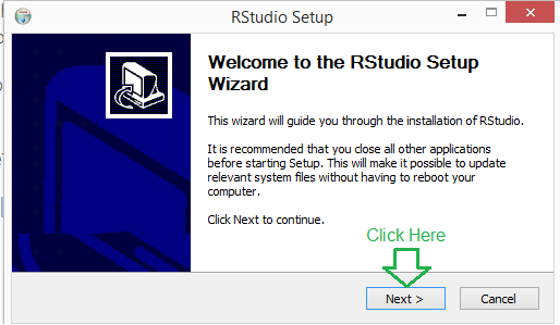
Figure 5.6 shows the start of the installation process. We will click on the "Next" button to move to the next step.
| Figure 5.6 |
|
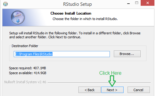
In Figure 5.7 we see that the installation program will allow us to choose the location for the actual software. The default location is provided and we can just accept that by clicking on the "Next" button.
| Figure 5.7 |
|
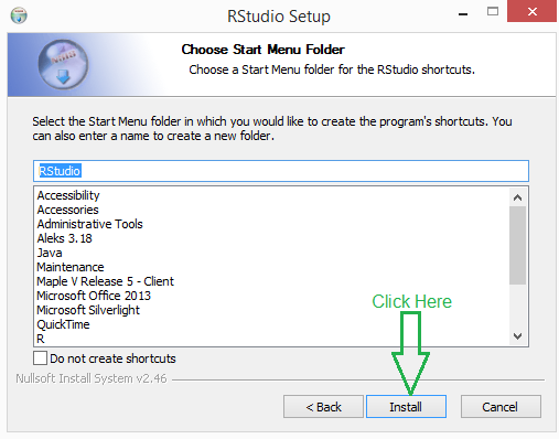
We can then choose if we want to locate the shortcut in some existing folder. Again, just click on the "Next" button.
| Figure 5.8 |
|
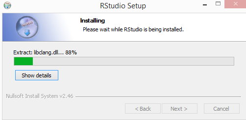
Figure 5.9 shows the progress display during the installation process. Once that is complete we will move to Figure 6.
| Figure 5.9 |
|
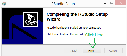
Figure 6 shows that the installation is complete and we click on the "Finish" button to acknowledge this and terminate the installation program.
| Figure 6 |
|
At this point RStudio has been installed. Now we want to run it. If we were going to run this just once in our life then we could take the inconvenient but consistent method of just searching for the program and then running it. However, we expect to run this program many times a day and on many days in the future. Therefore, we would like to have a readily available shortcut to start this program. Unfortunately, the methods for creating and locating such a shortcut are different in Windows 7, 8, and 10. As noted above, this particular installation was done on a Windows 8 machine. Similar, slightly easier though distinctly different, steps can be taken on Windows 7 and Windows 10 machines.
First, on this Windows 8 machine, we point to the lower right
corner of the screen to bring up
the options pane. In that pane we find the search option,
 , and then click on that icon.
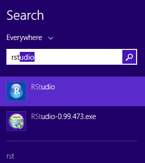
That action will open the "search pane" and we will start typing
"RStudio". In Figure 7, you can see that after
just 3 characters the
search is already suggesting both the completion of our typing and the two
files that it has found for us.
, and then click on that icon.
That action will open the "search pane" and we will start typing
"RStudio". In Figure 7, you can see that after
just 3 characters the
search is already suggesting both the completion of our typing and the two
files that it has found for us.
| Figure 7 |
|
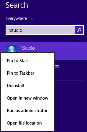
We want the "RStudio" item. If we want to just run this one time we could click on the item and start it. However, we would like to create a shortcut for running the program. Therefore, we point to the item and "right click" on it to open the sub-menu shown in Figure 8.
| Figure 8 |
|
We could click on "Pin to Taskbar", my favorite option, to place a shortcut item onto the taskbar". Or we could click on "Pin to Start" to place a shotcut on the "start menu". Or we could do one of those and then come back and do the other to have both options.
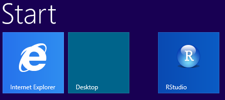
Just to illustrate, on this machine I clicked on the "Pin to Start", after which I went to the start menu and found, as shown in Figure 9, the shortcut to RStudio. To start RStudio just click on that icon.
| Figure 9 |
|
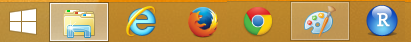
Alternatively, back in Figure 8, I could click on "Pin to Taskbar", in which case the shortcut to RStudio would appear on the Taskbar, as shown, from the PC I was using, in Figure 10. To start RStudio just click on that icon.
| Figure 10 |
|
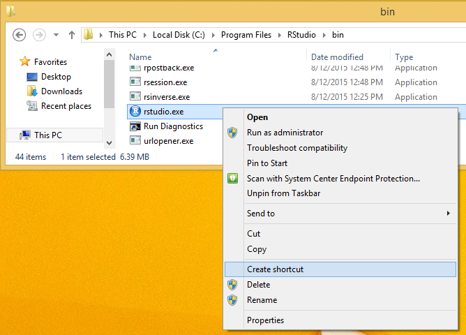
Yet another approach is to use the File Explorer to find the actual executable file for the RStudio program. Using the default values during the installation should mean that the executable file is in the "C:/Program Files/RStudio/bin" directory. In Figure 10.3 we have navigated to that directory and scrolled down to find the rstudio.exe file. [Your File Explorer may not be set to show the file extensions in which case this will just show as "rstudio" in the list.) Having found the file we click on it once and then "right click" on it to show the menu of actions displayed in Figure 10.3. Of those possible actions we choose "Create shortcut" and click on that option.
| Figure 10.3 |
|
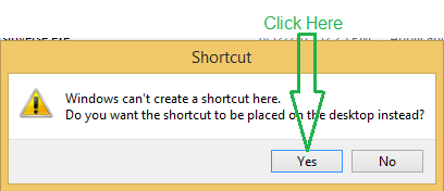
The system responds with a message, as shown in Figure 10.6, telling us that it cannot create the shortcut here and asking us if we want to create it on the desktop. This is exactly what we want to do so we click on the "Yes" button.
| Figure 10.6 |
|
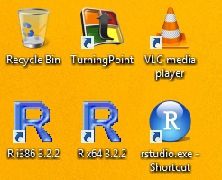
The result is a new shortcut on the desktop as shown in Figure 10.8 below. To start RStudio from that icon just double click on it.
| Figure 10.8 |
|
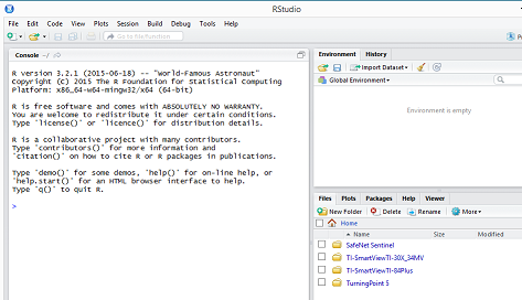
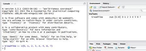
No matter which method we used, RStudio starts.
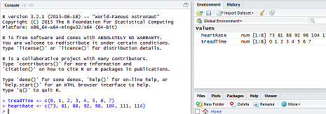
Figure 11 shows the initial screen for RStudio. We note that left pane inside RStudio is the "splash" screen for R. RStudio is an IDE for R. That means that we can use RStudio to interact with R, which we do directly in the left pane. We will see some of the uses of the other panes within the RStudio window in the following example.
In preparation for this example, I kept track of my heart rate each minute of the first 7 minutes of my standard exercise routine. Here is the recorded data:
| Time (in minutes) | 0 | 1 | 2 | 3 | 4 | 5 | 6 | 7 |
| Heart Rate | 73 | 81 | 88 | 92 | 98 | 104 | 111 | 114 |
| Figure 11 |
|
Our first action will be to get the data from the table into R. To do this we want to create a variable to which we can assign the values of the Time and another variable to which we can assign the values of the Heart Rate. Without getting into too much detail, we will use the command
treadTime <– c(0, 1, 2, 3, 4, 5, 6, 7)
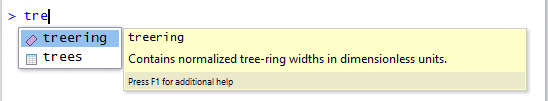
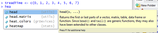
Figure 12 shows the system reaction to our typing just the first three letters of that command.
| Figure 12 |
|
The extra information displayed in Figure 12 is RStudio trying to help us. Sometimes, as in this example, that help is not appropriate, but RStudio does not know this. It is just trying to help. It is saying,
| By the way, there are two special words that I know that start with 'tre', namely 'treeing' and 'trees', and if you want to save some typing, here they are for you to select. And, just so that you know, 'treeing' Contains normalized tree-ring widths in dimensionless units. |
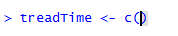
We get as far as typing
treadTime <– c(
| Figure 13 |
|
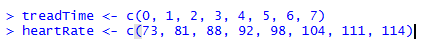
We just keep typing in our command until it is completed, as shown in Figure 14.
| Figure 14 |

|
At that point we press the Enter key to tell R to perform the command. The result is shown in Figure 15. Notice that the only thing that happens in the left pane is that we get another prompt, the > sign. However, the top right pane now shows us that we have a variable, named treadTime, and that variable has the indicated values. This confirmation and display of the entities and their values that now exist in our R session is extremely useful.
| Figure 15 |
|
We will continue by typing the command
heartRate <– c( 73, 81, 88, 92, 98, 104, 111, 114)
| Figure 17 |
|
(There is no Figure 18 )
(There is no Figure 19)
We complete the command so that we have entered
the commands as shown in Figure 20.
| Figure 20 |
|
To get to Figure 21 we hit the "Enter" key to tell R to perform the command. R did not find a problem with our requested action so it performed it. RStudio, which monitors R confirms this by displaying the new variable, heartRate, and its initial values in the top right pane.
| Figure 21 |
|
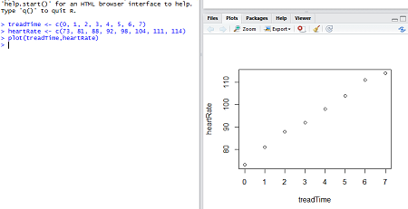
We can show off a little bit by asking R to create a scatter plot of the treadTime values against the heartRate values. To do this we just type
plot(treadTime, heartRate)
| Figure 22 |
|
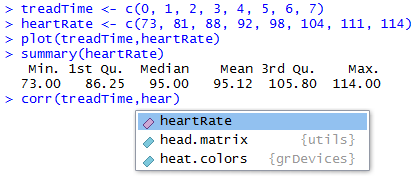
How about another R command:
summary(heartRate)
   Min. 1st Qu.  Median    Mean 3rd Qu.    Max.
  73.00   86.25   95.00   95.12  105.80  114.00
Thus, in one simple command we learn the minimum value, 73, the maximum value, 114, the median (or middle) value, 95, the mean (numerical average) value, 95.12, the first quartile (25th percentile) value, 86.25, and the third quartile (75th percentile) value, 105.8.
| Figure 23 |
|
Figure 23 concludes with an attempt to submit another command. In the process of typing this command, in the middle of typing heartRate, the system is offering "heartRate" as a suggestion to complete the typing. To accept that offer, we just need to press the "Enter" key. That will take us to Figure 24.
A careful observer will notice that the "vertical insertion bar" is missing in that last line of Figure 23. It really is not so much missing as it was not captured when the screen image was taken. The vertical bar "flashes" and if it is not present when the image is captured then it will not be in the image. That is what happened in Figure 23. There really was a vertical bar between the "r" and the ")" in that line, and you would see it flashing if you did this on your machine.
| Figure 24 |
|
There are a few ways we can finish entering the command seen at the bottom of Figure 24. First, we could type the right parenthesis. RStudio knows that it supplied the right parenthesis already displayed in Figure 24, so our new right parenthesis will just replace that one. second, we could use the cursor controls or the mouse to move the insertion point beyond the right parenthesis. In either of those two cases our next action would be to press the "Enter" key. Our third option would be to just press the "Enter" key. RStudio would just assume that we wanted to complete the command with the right parenthesis that it supplied.
Use any of those methods to complete the command and ask R to execute it.
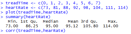
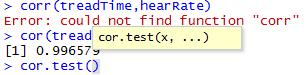
The first line of Figure 25 is the command we entered.
The second line of Figure 25 is the error message that R gave to us because the line we entered was incorrect. There is no predefined function called "corr" in R. Getting an error message like this is actually quite common. It just means that we have to fix what we entered.
The correct line
cor(treadTime,heartRate)
| Figure 25 |

|
We conclude Figure 25 by starting to type the command
cor.test(treadTime,heartRate)
| Figure 26 |
|
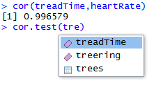
Then, as we start to type "treadTime" RStudio again offers to complete our work, suggesting "treadTime". Again, press the "Enter" key to accept that offer.
| Figure 27 |
|
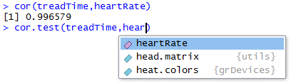
Figure 28 shows that RStudio has filled in "treadTime", and we have continued with ",hear", at which point RStudio is again trying to help by suggesting three things. In Figure 28 the second option is highlighted. We want the first so we could click on that, or we can just keep typing away ourselves.
| Figure 28 |
|
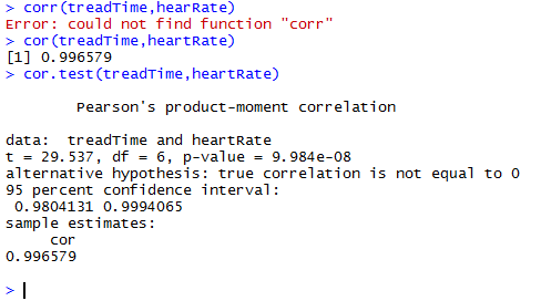
Either way, we finish the command and press the "Enter" key. This produced the multi-line output shown in Figure 29. Here we have lots of answers generated by our one simple command.
| Figure 29 |
|
You may notice that the last three lines of the output shown in Figure 29 give exactly the same simple answer that we got earlier from the "cor" function in Figure 25.
| Figure 30 |

|
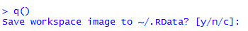
We conclude Figure 30 with the "q()" command to ask R to quit. R responds by asking if we want to "Save workspace image to"? We can respond to this by typing "y" for "yes", "n" for "no", or "c" for "cancel the quit request".
Remembering that this web page is just meant to demonstrate some of the features of R and of RStudio, we will respond with "y" to cause the program to quit but to save the workspace.
| Figure 31 |
|
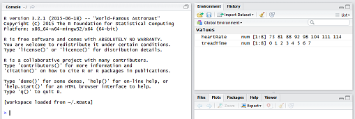
Saving the workspace means that we can restart R or restart it through RStudio, and it will pick up right where we left off. Let us try that. We will restart RStudio using the same method we did back between Figure 8 and Figure 9.
| Figure 32 |
|
There are two things to notice in Figure 32. First, toward the bottom of the "splash screen" shown in the left pane, R is telling us that
(Workspace loaded from ~/.RData). Second, in the upper right pane we see that the two variables that we had created before, namely,
treadTimeand
heartRatehave been restored. Thus, we could pick up our work right where we left off.
©Roger M. Palay
Saline, MI 48176 August, 2015