RStudio — PC Install and More

This page is based on the installation of RStudio on a PC computer using the Firefox web browser. The process took place on August 17, 2015. The standard version of RStudio at that time was 0.99.467. Please understand that web pages change, software changes, and installation systems change. Thus, what is recorded here, although true at the moment of recording, may have changed by the time you read this.

Also, as I hope is obvious, the images below have been annotated, in GREEN, to show you where you need to point and click.

Just a few quick notes:

We will short-circuit the installation by starting not at the RStudio main web page but rather right at the point where we choose the file to use.
The installation of the software is done in Figure 11.
Following the installation there are sections of this page showing three different ways to start the software. A fourth method, and the one that you will most likely use most often, appears starting in Figure 37.
Starting in Figure 27 we do one quick use of RStudio. This gives us a chance to examine some of the components of the IDE (Integrated Development Environment).
Many of the Figures have been shrunk to facilitate display and printing. This should not compromise the readability of the images; the images are really just there to verify and explain what you should be seeing on your screen.
This material has not been formatted for printing so if you do print it you will get a lot of blank space and the Figure numbers may be separated from the images by page breaks.

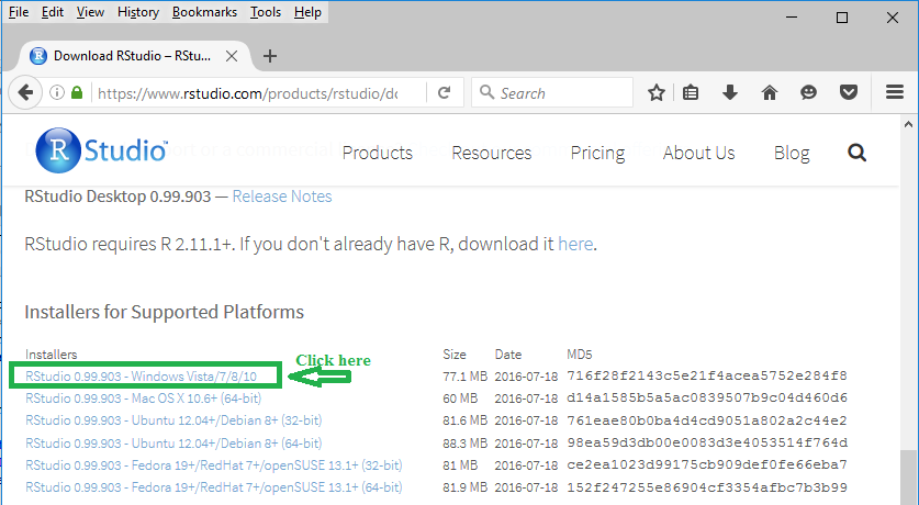
To install RStudio, we will go to the RStudio web site at the https://www.rstudio.com/products/rstudio/download2/#download web site. This should open a page almost identical to the one shown in Figure 1. For a PC we want to use the RStudio 0.99.903 - Windows Vista/7/8/10 option, the one highlighted by the green box in Figure 1.

Figure 1

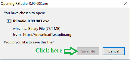
The particular installation of Firefox used here was set to ask the user where downloaded files should be saved. The version that you use may or may not be similarly configured. That will not matter since we will use a different feature of Firefox, in Figure 4, to run the downloaded file no matter where it has been saved. [A similar feature exists an any of the other modern browsers.] Firefox first asks if we want to Save File, as shown in Figure 2. We do want to save the file so we click the Save File button.

Figure 2

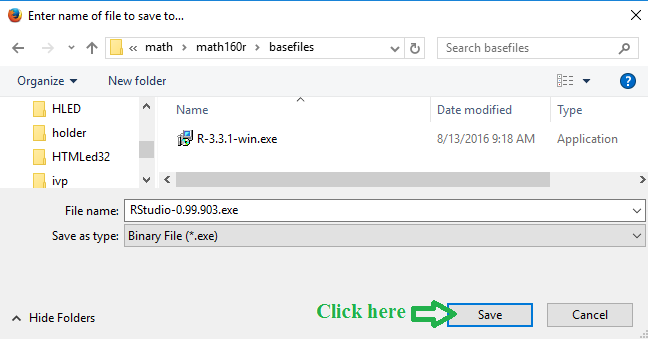
As just noted, the version of Firefox here wants to have us determine where to save the file. In the case shown here it will be saved in the directory structure C:/math/math160r/basefiles although the particular place is immaterial to this presentation. If you see a window such as that shown in Figure 3, just click on the Save button.

Figure 3

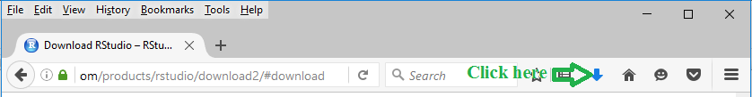
Once the file is downloaded to your computer we need to run the file. On the top bar of the Firefox screen we find the down arrow,

, icon as highlighted in Figure 4.

Figure 4

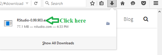
When you click on that icon, a new window shows up displaying the recent downloads. In Figure 5 we see the RStudio-0.99.903.exe file that we just downloaded. To run that file we click on the file name as indicated in Figure 5.

Figure 5

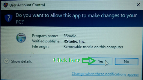
At this point, on this computer using Windows 10, the operating system wants to get a confirmation that it is OK to actually run the program that we downloaded. [Note that running a downloaded program is possibly dangerous if the original site had a corrupted or infected file waiting for you.] In this case we are confident that the source of our file is to be trusted so we click the Yes button.

Figure 6

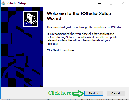
The install program starts. We will just step through the options. Figure 7 shows the first screen and we move on by clicking the Next button.

Figure 7

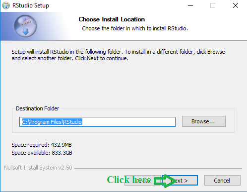
The same is true for the window shown in Figure 8.

Figure 8

The same is true for the window shown in Figure 9. However, it is worth noting that the installation program, in Figure 9, is asking about the location of the program's shortcut. By not making any changes here we instruct the installation program to put that shortcut into the Start menu. We will see this in Figure 26 .

Figure 9

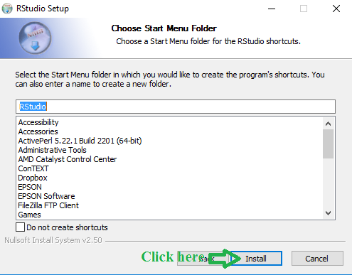
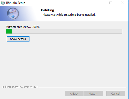
Figure 10 catches the install progress screen as the installation continues.

Figure 10

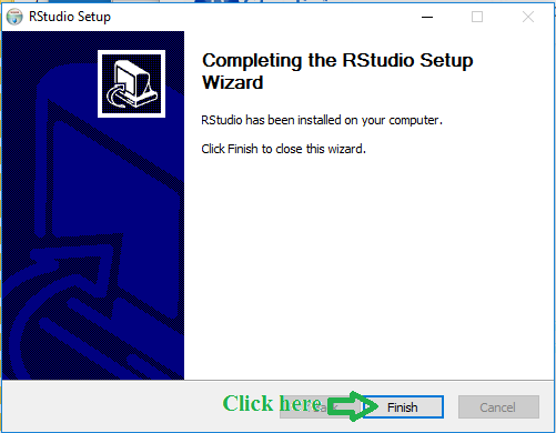
Finally, in Figure 11, the installation is complete and we can click the Finish button to move forward.

Figure 11

Now that RStudio has been installed, we want to be able to run it. The presentation from here through Figure 26 demonstrates three different ways to start RStudio, either directly from the Start menu or from an icon that you can put onto your desktop. These are interesting but not essential for this course. The suggested method for this course starts after Figure 37. The presentation from Figure 27 through Figure 36 just walks us through a short problem, allowing us to point out different features of the RStudio environment.

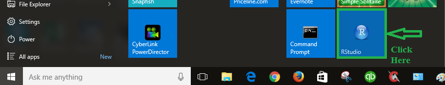
Back in Figure 9 we had the installation program place the shortcut for RStudio onto the Start menu. If we open that menu either by clicking the Windows icon,

, at the extreme lower left of the screen or by typing the Windows key on the bottom left of the keyboard, we will get a new window. Part of that window on my computer is shown in Figure 12 (after scrolling down to display the desired shortcut,

).

To start RStudio just click on that shortcut, as shown in Figure 12.

Figure 12

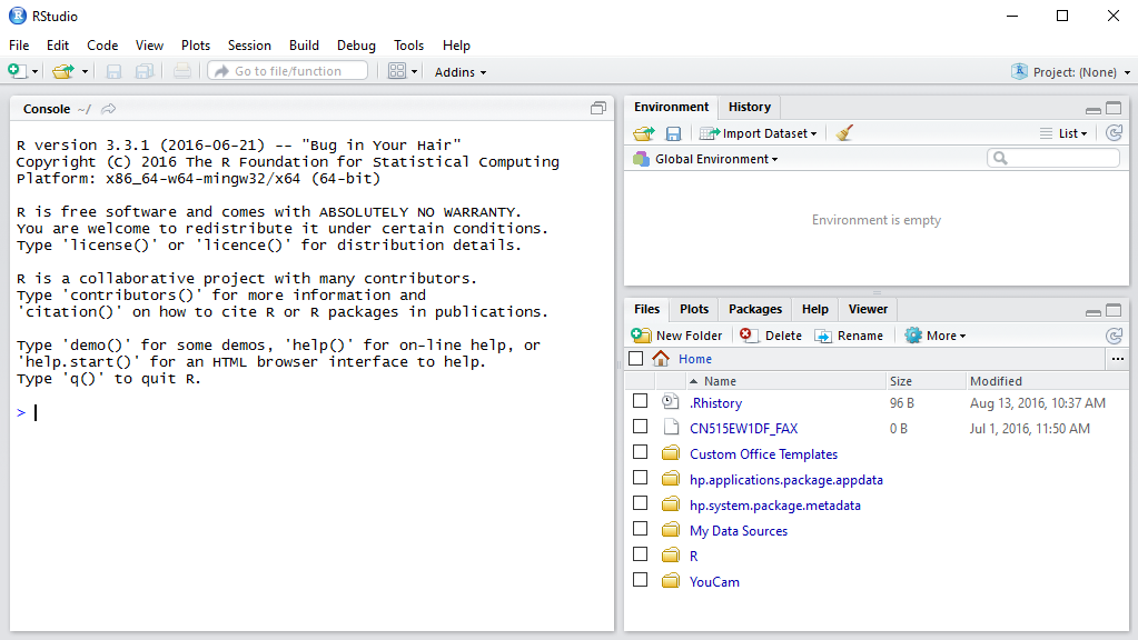
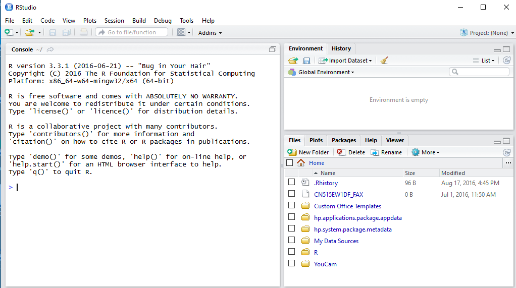
RStudio opens as shown in Figure 13. The RStudio window is divided into 3 panes, the Console, the Environment (which can alternatively display the History), and the Files (which has a number of other options).

Figure 13

We will come back to this in Figure 27. Before we do that, however, we will look at two ways to put the shortcut icon onto the desktop.

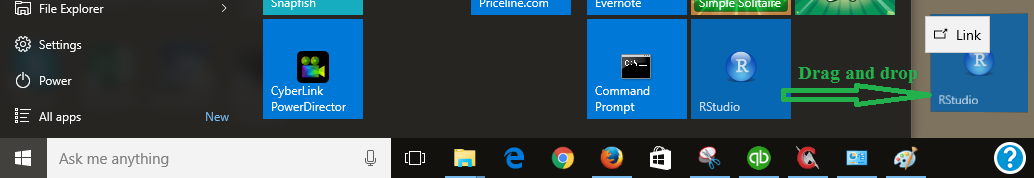
The most straightforward way is to return to the Start menu, find the shortcut for RStudio, then click and hold on that shortcut and drag it to the desktop where we release the mouse button. This is shown in Figure 14.

Figure 14

Once the shortcut icon is on the desktop we can just double click it to start RStudio.

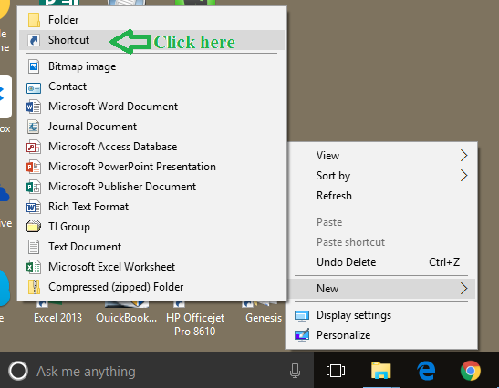
A much more tedious method to create the shortcut is to start at any open spot on the desktop and right-click the mouse. This opens a small window, one option on which is New. Put the cursor on that New option and, shortly, a secondary window opens, as shown in Figure 15. Point to the Shortcut option in that window and click there.

Figure 15

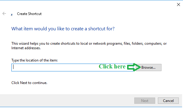
We could type in the location of the file but we will take the slightly longer if somewhat safer approach of looking for it. To that end click on the Browse button.

Figure 16

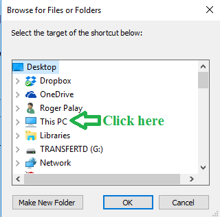
We want to look on This PC, so click on that.

Figure 17

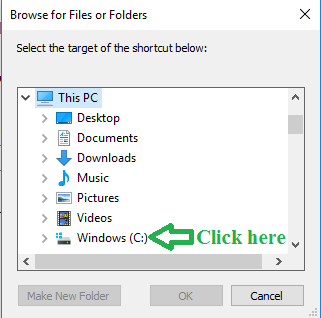
We want to look on the C drive, so click on that.

Figure 18

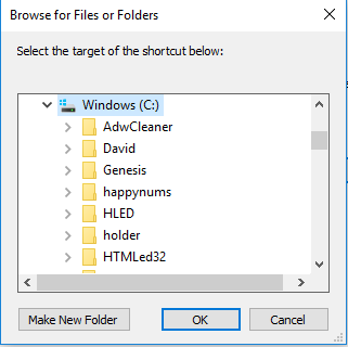
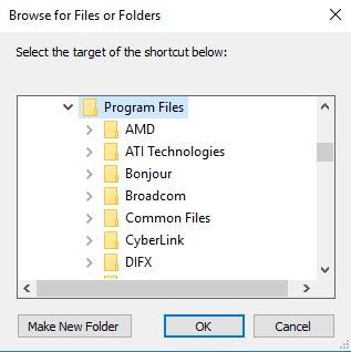
Next we want to look in Program Files but that is not shown in Figure 19.

Figure 19

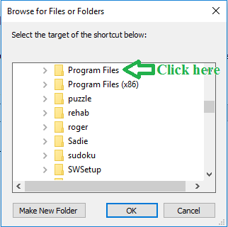
Therefore, scroll down to find Program Files, as shown in Figure 19a. Once we have found it, then click on that item.

Figure 19a

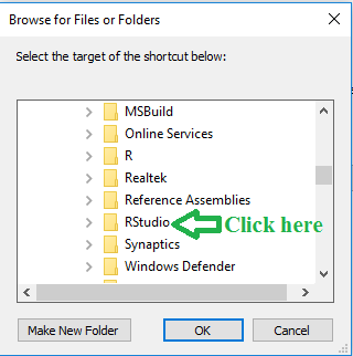
Now we want to find RStudio, but again it is not yet visible in Figure 20.

Figure 20

Therefore, scroll down to display RStudio as shown in Figure 20a, and then click on that item.

Figure 20a

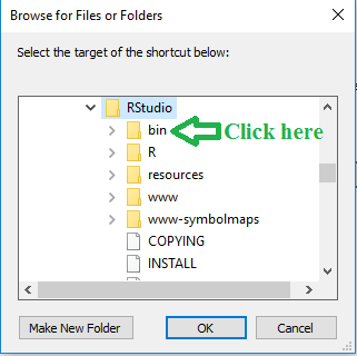
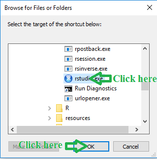
Now click on the Bin item.

Figure 21

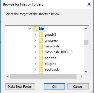
In this window we want to find the rstudio.exe option. It is not shown in Figure 22.

Figure 22

Therefore we scroll down to find it, and click on it as shown in Figure 23. At that point we click on the OK button.

Figure 23

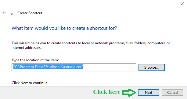
This takes us back to the window that we saw back in Figure 16 but now the location field is filled in, and it is filled correctly. All we need to do now is to click the Next button.

Figure 24

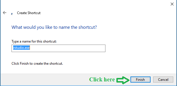
This brings up our final screen where we click on the Finish button.

Figure 25

The result is a new shortcut, shown in Figure 26, on the desktop.

Figure 26

Once we have the desktop shortcut, we just need to double click on it to start RStudio. We have done so in order to get the RStudio window shown in Figure 27 (which is the same as the one we saw in Figure 13.

Figure 27

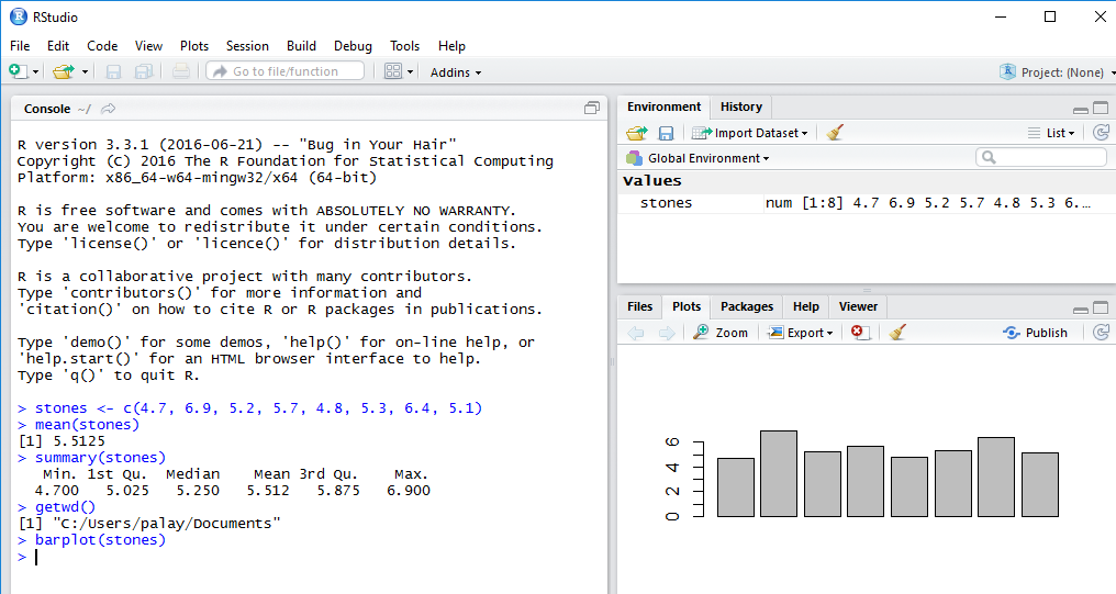
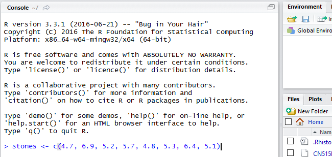
As long as we have started RStudio we might as well try it out. We have the following problem. Walking around near the parking lot I found and collected 8 stones. I then weighed those stones and obtained the following measurements.

Weight of the stones I found
4.7	6.9	5.2	5.7	4.8	5.3	6.4	5.1

We want to put those values into RStudio. To do this, in the Console pane, we enter the command
stones <- c(4.7, 6.9, 5.2, 5.7, 4.8, 5.3, 6.4, 5.1)
in the Console after the > prompt.. This produces the image shown in Figure 28.

Figure 28

Now, to have R perform the command, we hit the Enter key on the keyboard. The result is shown in Figure 29.

Figure 29

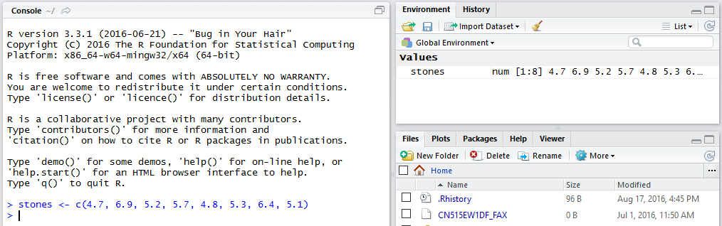
Our command has caused R to create a variable called stones, and to assign that variable the list of values that we specified. The Environment pane monitors the variables that have been defined. It also displays the first values stored in those variables. We only have the one variable so far, but we can see it, the fact that it is num meaning numeric, that it has eight values in it (items 1 through 8), and the value of the first few of those items.

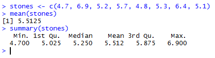
Let us do two more operations on the data. First we will ask R to find the mean (the average of the values, i.e., add up the values and divide by the number of values), and second, we will get a summary of the values. The first command is
mean(stones)
which we enter and then press the Enter key. R responds with the value 5.5125. The second command is
summary(stones)
which produces six values: the lowest value in the data, the 1^st quartile, the median value, the mean value, the 3^rd quartile, and the largest value in the data. You might note that R gives these with only 3 decimal places whereas R gave the mean value with 4 decimal places.

Figure 30

A completely different kind of command is getwd() shown in Figure 31. That command is a function that retrieves the working directory that R and RStudio are using at that time.

Figure 31

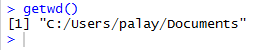
The result of using the command is C:/Users/palay/Documents, indicating that as the location of any files that we are using or that we might want to save. More on that later.

We can demonstrate yet another type of command, namely,
barplot(stones)
shown in Figure 32. The result of that command is a new plot, shown in the lower right pane, that is a bar plot of the data held in the variable stones.

Figure 32

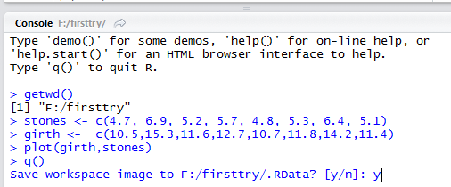
Finally, we use the q() command to tell R and RStudio to quit. For Figure 33 we have typed the q() command and pressed the Enter key. R then asks us if it should save the "workspace". This is also shown in Figure 33.

Figure 33

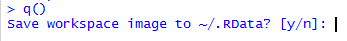
We want to save the workspace, so we answer "y" and press the Enter key. After that our RStudio session is closed.

[Figure 34 is omitted.]

By "saving the workspace" we have told R to save all of our variables in a "hidden" file called .RData, and to save that file in the "working directory". We can see this if we open RStudio again (by double clicking on the RStudio icon on the desktop). We have done this to generate Figure 35.

Figure 35

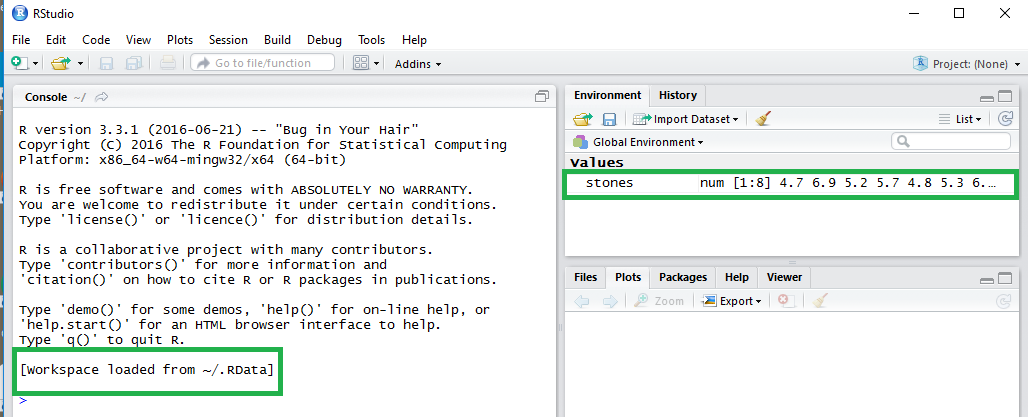
Two things to note in Figure 35 are the new last line of the "splash" screen from R telling us that the workspace has been loaded from the file and the fact that the one variable we had in our previous session is still defined.

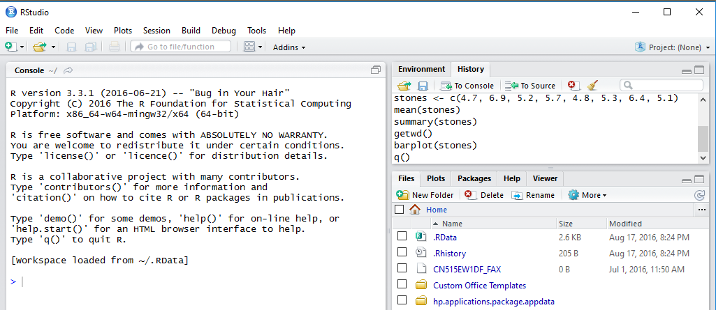
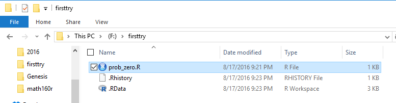
In fact, if we click on the Files tab in the lower right pane we change the display to that shown in Figure 36. In that pane we can see that the file .RData is now in that directory, that the file size is 2.6KB, and that it was created on Aug. 17 at 9:24 PM. In fact, a new history file called .Rhistory was created at that same time, the moment when we closed our previous session.

Figure 36

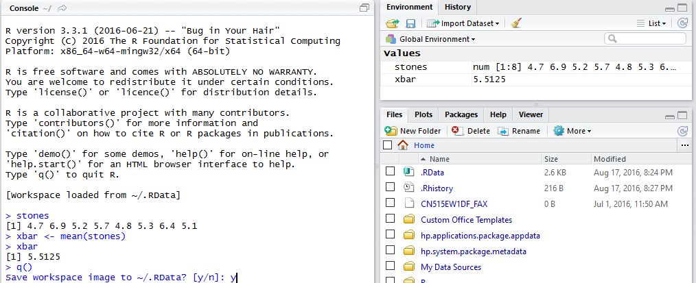
We will finish this introduction with a few more commands shown in Figure 37 along with the resulting output from R. First, the command stones causes R to display the contents of the variable stones. Then the command
xbar <- mean(stones)
has R compute the mean and then store that value in the new variable xbar. Note that R does not display the value of xbar at that time, although RStudio displays it in the Environment pane. Then the command xbar causes R to display the value stored in the variable. Finally, the command q() causes R to ask if it should save the workspace. Again we respond with y. Once we press the Enter key the program will save the workspace and close.

Figure 37

At this point we will shift gears and look at the preferred, and expected, method of opening a new RStudio session. To do this we will plug in the USB thumb drive given out in class. When I did this on my computer the response was to open the File Explorer to display the contents of the USB drive. This is shown in Figure 37a.

Figure 37a

Although it is nice to see the contents of the USB drive, at this point we will not be making reference to the existing files. Therefore, at this time we can close the File Explorer by clicking on the X in the upper right corner of the window.

Our approach will be to create a text file that contains just the command getwd() and then to save that file in a subdirectory of the USB drive that we will create. Then, we can return to the File Explorer, navigate to that subdirectory, and start a new RStudio session by double clicking on the name of our new file.

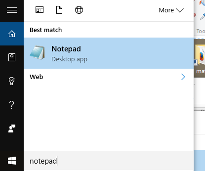
We could do this in any number of different text editors but because it is available on any Windows system, we will use Notepad. To find and start Notepad we can just type notepad into the "Ask me anything" box at the lower left of the screen. The result should be something similar to what is shown in Figure 38.

Figure 38

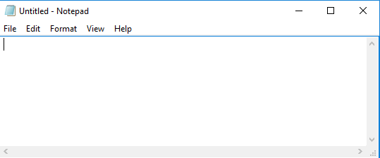
Click on the Notepad icon and the program should start with a screen similar to that shown in Figure 39.

Figure 39

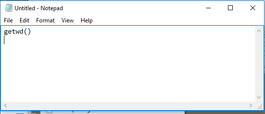
Now type the one text line, namely, getwd() and press the Enter key to move to a new line. This should show up as in Figure 40.

Figure 40

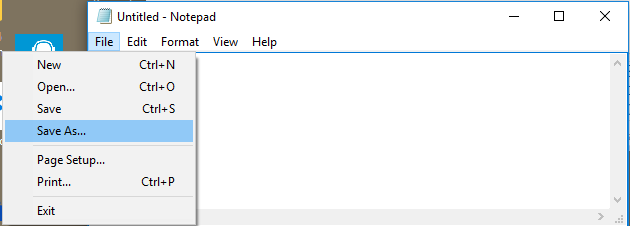
Then, from the menu bar choose the File option and from the new window click on the Save As... option, as appears in Figure 41.

Figure 41

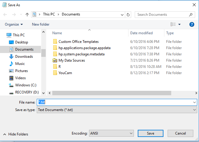
This will open a window similar to that shown in Figure 42. In the left pane of Figure 42 we want to find the entry for the USB thumb drive that we just installed.

Figure 42

On this computer we could not see that entry so we needed to scroll down that left pane. Figure 43 now displays that drive as USB Drive (F:). We click on that entry producing the display given as Figure 43.

Figure 43

None of the files that we saw back in Figure 37a appear here because this window, the one shown in Figure 43, is looking for all of the "Text" files, the ones with the .txt extension. There are none of those files on the USB drive.

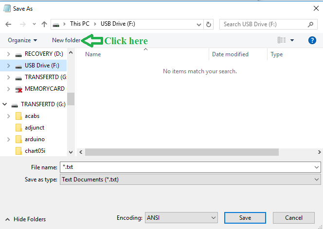
However, our task is not to find a file, but to save one in a new folder. To that end we click on the New Folder button.

Figure 44

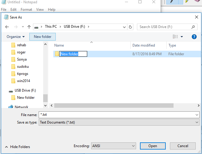
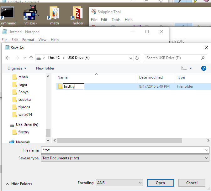
This creates a new folder and it suggests the name New Folder for that directory. We, however, will call this folder firsttry and we do that by typing that name into the given box as shown in Figure 45.

Figure 45

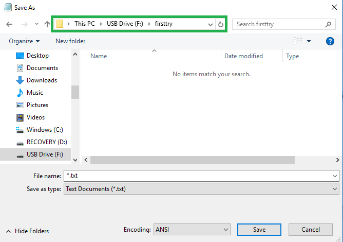
Once the folder has been created, we still need to navigate to it. We can do this by double clicking on the folder icon

to the left of the name. This should bring us to the image in Figure 46. Note, in the location bar near the top of Figure 46, that we are in the proper subdirectory.

Figure 46

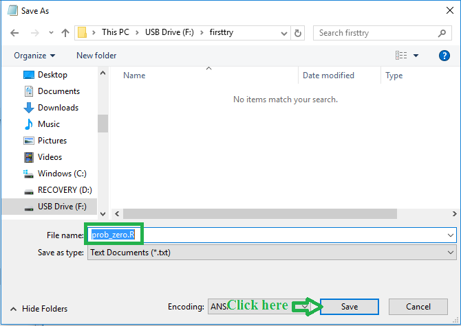
Now that we are there we can enter the name of our new file, I have called it prob_zero.R and please note that it is important to have the file extension be .R in this case. We conclude the process of saving the file by clicking on the Save button.

Figure 47

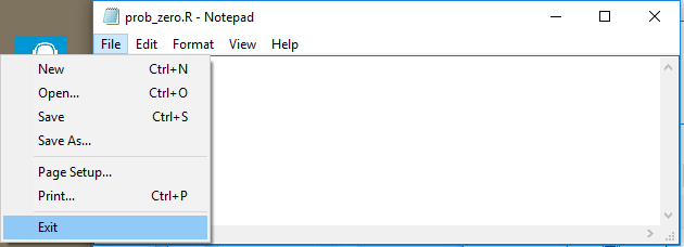
That leaves us in Notepad. To exit the program we click on the File option in the menu and then click on the Exit option in the small window that opens.

Figure 48

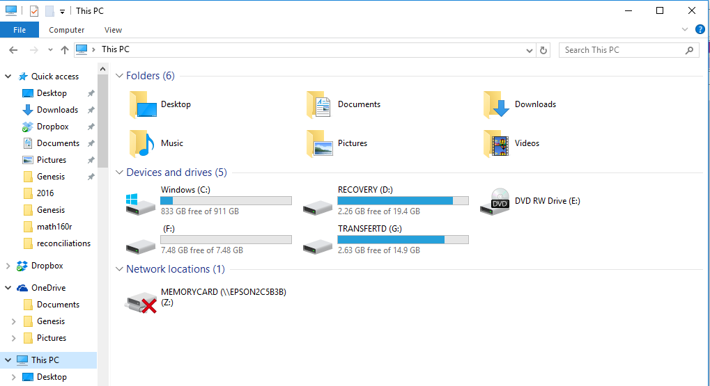
Recall that the next step is to find our newly created folder and the file in it via the File Explorer. To do that we start the File explorer by clicking on the folder option at the bottom of the screen, as is shown in Figure 48a.

Figure 48a

Then we can navigate to This PC by clicking on that item in the left pane, and to the F drive shown on the window.

Figure 49

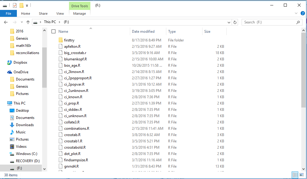
All of that should change the display to something like that shown in Figure 50. Once there we can open the folder by clicking on the firsttry entry.

Figure 50

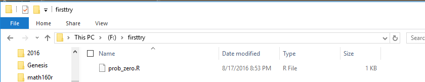
This should take us to Figure 51. There we can see the file that we just created. We will double click on that filename, prob_zero.R.

Figure 51

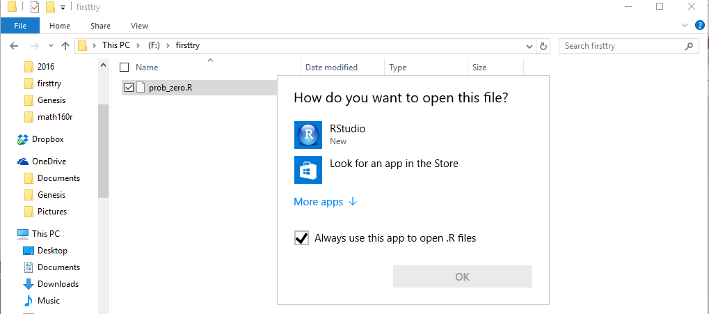
This being the first time we have tried this, the computer asks for help in determining which program should be used to open files that have a .R extension. It does this via a pop-up window like the one shown in Figure 52.

We want to use RStudio so we will make sure it is highlighted (we may need to click on it to do that).

Figure 52

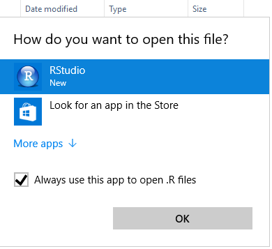
After the RStudio option is highlighted we should be sure that the checkbox for Always use this app to open .R files is marked, as it is in Figure 53. Then we can click on the OK button.

Figure 53

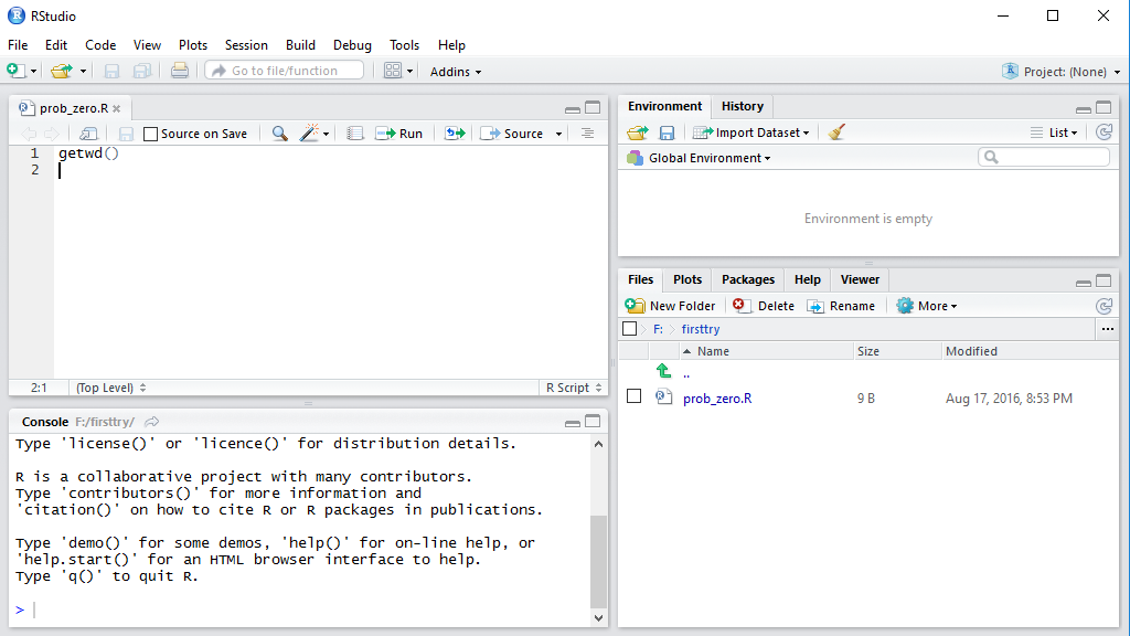
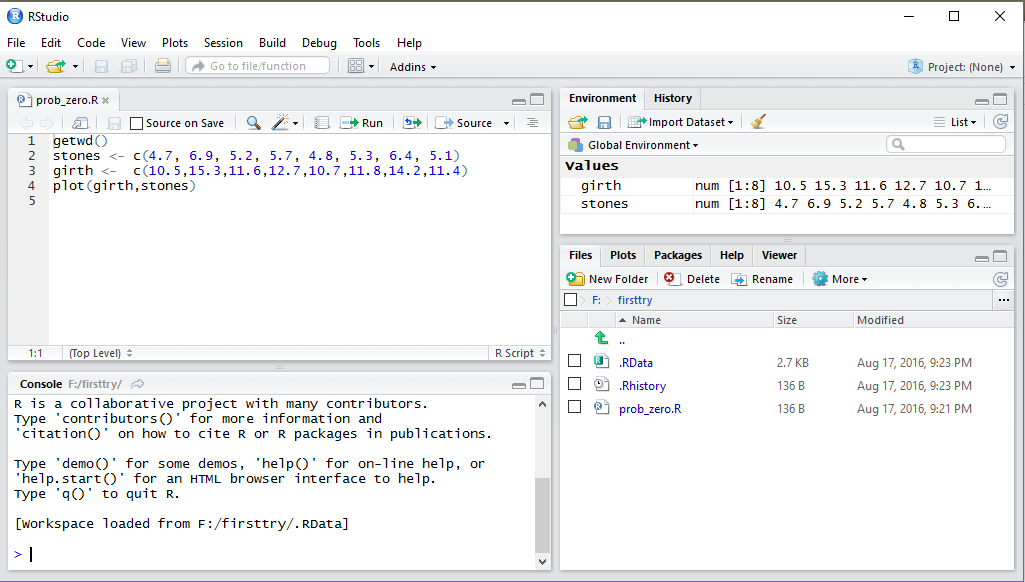
That starts RStudio. This time the RStudio screen is split into 4 panes. The new pane is an editor, built into RStudio, that has not only opened, but it has opened with our file in it.

Having a file into which we can type commands and then, as we will see, execute those commands is a significant advantage. Among other things, it allows us to take our work to another computer, to share our work with others, and to record and publish our work. This is an essential skill that all statisticians need to have.

Figure 54

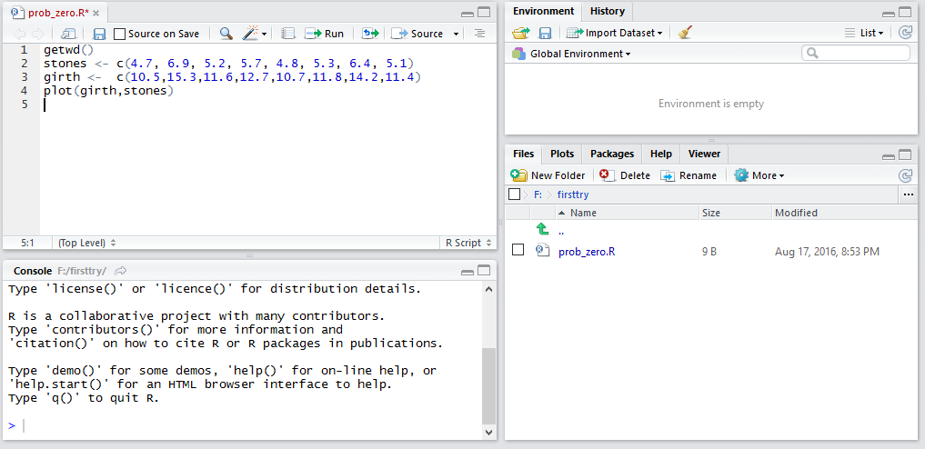
To demonstrate this, in the editor pane, type the following commands

getwd()
stones <- c(4.7, 6.9, 5.2, 5.7, 4.8, 5.3, 6.4, 5.1)
girth <-  c(10.5,15.3,11.6,12.7,10.7,11.8,14.2,11.4)
plot(girth,stones)

Actually, if you have this page open and you have your RStudio session open as shown in Figure 54, you can just highlight the commands above, copy them via the ctrl-c key sequence, click on the editor pane, and paste the commands via the ctrl-v key sequence. This saves a lot of typing. Your editor pane should appear as in Figure 55.

Figure 55

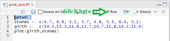
Now, to demonstrate executing commands that are in the editor, highlight the getwd() command, as shown in Figure 56. Then click on the Run icon,

, on the editor toolbar, indicated in Figure 56.

Figure 56

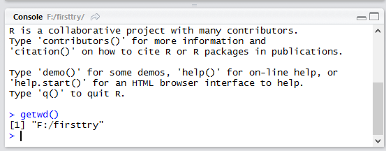
The result appears in Figure 57. The command has been copied to the Console and performed. It is interesting to note that the working directory for this session is our newly created folder. This is just what we want. When we save the workspace later the files .RData and .Rhistory will be saved in this directory. In that way we are keeping all of our work related to our current problem in one folder.

Figure 57

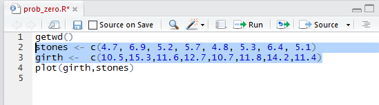
Returning to the editor, we can highlight our next two commands as shown in Figure 58. Then, we can again click on the run icon,

, on the editor toolbar to copy those commands to the Console and execute them.

Figure 58

The result is shown in Figure 59.

Figure 59

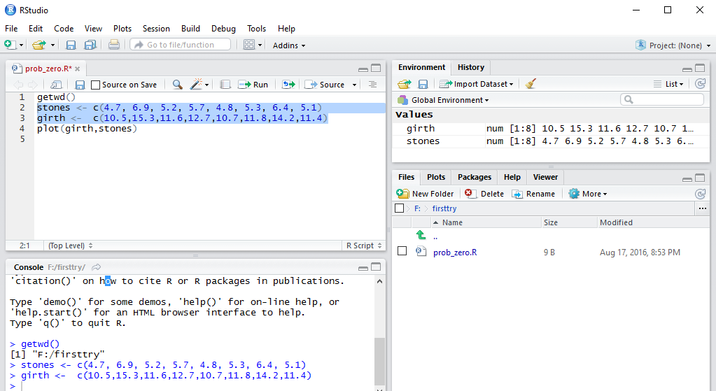
In Figure 59 we not only see that the commands have been performed, but the two new variables appear in the Environment pane.

To get to Figure 60 we need to highlight our last command in the editor pane and then use the run icon to cause the command to be copied and executed.

Figure 60

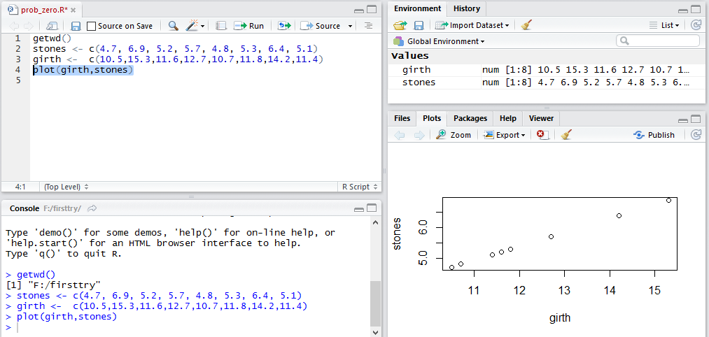
In Figure 60 we can see the plot created by our simple command.

By creating the plot we have automatically switched the lower right corner pane to the Plots tab. We can click on the Files tab in that pane to change the display to be more like that shown in Figure 61.

Figure 61

You may notice, in Figure 61, that we still have but one file in our folder.

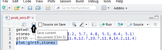
We return to the editor pane and click on the

icon to force saving the changes we have made in the file in the editor. This is shown in Figure 62.

Figure 62

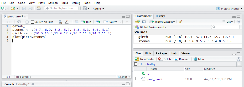
Once that is done we can turn our attention back to the File pane where we see that the file is now bigger, 136 bytes vs. the earlier 9 bytes, and the time stamp has been updated.

Figure 63

We can return to the Console where we issue the q() command and then say that we do want to save the workspace, all shown in Figure 64.

Figure 64

Once we conclude that with the Enter key, RStudio closes.

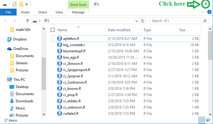
Returning our attention to the File Explorer, shown in Figure 65, we can see the two new files.

Figure 65

If we double click on our prog_zero.R file again, RStudio starts anew. Figure 66 shows this new session. Note that the splash screen shows that the workspace was loaded from our folder, that the file has been loaded into the editor, and that the two variables that we defined are available as shown in the Environment pane. In addition, we can see the three files in the Files pane.

Figure 66

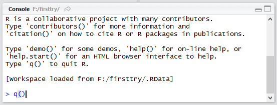
As usual, we use the q() command to quit RStudio.

Figure 67

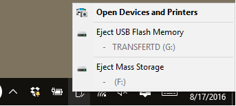
All that remains now is to remove our USB drive. It is a good idea to make sure that the computer thinks it is ok to do this. If the

icon is present at the lower right of your screen then click on it. If it is not present, then you may have to click on the up-arrow, shown in the red circle in Figure 68, to find the

icon.

Figure 68

This should open a window listing the various devices that can be removed. Such a list appears in Figure 69. Click on the desired item.

Figure 69

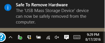
The response should be the small window shown in Figure 70. At that point it is safe to remove the USB drive.

Figure 70

Return to Software Installation