| Figure 1 |
|
|
This page is based on the installation of RStudio
on a Mac computer using the Firefox web browser.
The process took place on August 10, 2015.
The standard version of RStudio
at that time was 0.99.467.
Please understand that web pages change, software changes,
and installation systems change. Thus, what is recorded here,
although true at the moment of
recording, may have changed by the time you read this.
Also, as I hope is obvious, the images below have been annotated, in GREEN, to show you where you need to point and click. Just a few quick notes:
|
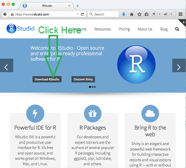
To install RStudio, we will go to the RStudio web site at the https://www.RStudio.com/ web site. This should open a page, the top of which should appear as shown in Figure 1.
| Figure 1 |
|
|
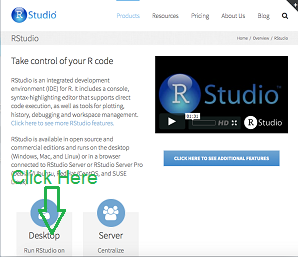
We will click on the "Download RStudio" button, as shown in Figure 1. Most likely, the result will be the screen shown in Figure 2. Your only clue as to the next step is to click on the "Desktop" version. That is the action suggested here. [However, if you just point the that same "Desktop" icon, you will see that it is just a link, https://www.RStudio.com/products/RStudio/#Desktop, to the same web page, just further down the page than we are in Figure 2. That is, you could just scroll down and get to the same place.]
| Figure 2 |
|
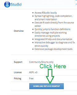
The result of your navigation should be the screen shown in Figure 3. You may need to scroll down to find the "DOWNLOAD RStudio DESKTOP" button. Then, click on that button.
| Figure 3 |
|
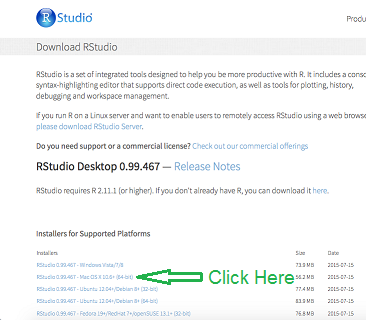
On this screen, the one shown in Figure 4, you finally get to make the choice of the version of RStudio to install. We, of course, want to select the "RStudio 0.99.467 – Mac OS X 10.6+ (64-bit)" option.
[Note that you could have just started at this page if you had used the URL https://www.RStudio.com/products/RStudio/download/ to start.]
| Figure 4 |
|
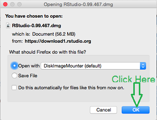
The computer responds with the screen shown in Figure 5. Our response is to just click on the "OK" button.
| Figure 5 |
|
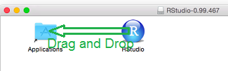
The RStudio program is downloaded and installed on the computer. We are then given the chance to see this and, if we want, to move the program into the applications. We want to do this. Therefore, starting in Figure 6, click on the RStudio icon and drag and drop it to the Application folder.
| Figure 6 |
|
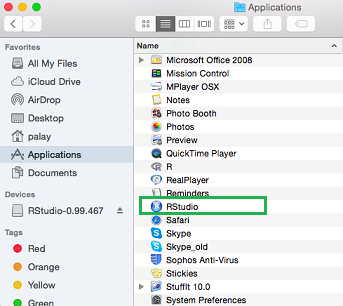
RStudio is now an application. Therefore, we have some options before us.
| Figure 7 |
|
If you opted for the second or third choice then the icon that will appear on the Desktop or in the quick start bar will be the one shown in Figure 8.
| Figure 8 |

|
The first time that you actually start RStudio on the computer most likely you will have to go through the following two screens.
Start RStudio now, using any of the methods noted above.
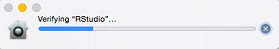
The computer first verifies the software, as shown in Figure 9
| Figure 9 |
|
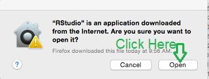
Then, just to be sure, the computer asks us if it is OK to run this given that we got it from the web.
Our response is to click the "Open" button.
| Figure 10 |
|
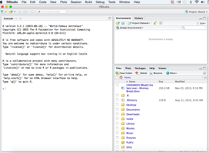
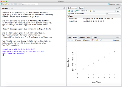
Figure 11 shows the initial screen for RStudio. We note that left pane inside RStudio is the "splash" screen for R. RStudio is an IDE for R. That means that we can use RStudio to interact with R, which we do directly in the left pane. We will see some of the uses of the other panes within the RStudio window in the following example.
In preparation for this example, I kept track of my heart rate each minute of the first 7 minutes of my standard exercise routine. Here is the recorded data:
| Time (in minutes) | 0 | 1 | 2 | 3 | 4 | 5 | 6 | 7 |
| Heart Rate | 73 | 81 | 88 | 92 | 98 | 104 | 111 | 114 |
| Figure 11 |
|
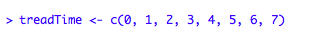
Our first action will be to get the data from the table into R. To do this we want to create a variable to which we can assign the values of the Time and another variable to which we can assign the values of the Heart Rate. Without getting into too much detail, we will use the command
treadTime <– c(0, 1, 2, 3, 4, 5, 6, 7)
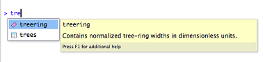
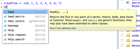
Figure 12 shows the system reaction to our typing just the first three letters of that command.
| Figure 12 |
|
The extra information displayed in Figure 12 is RStudio trying to help us. Sometimes, as in this example, that help is not appropriate, but RStudio does not know this. It is just trying to help. It is saying,
| By the way, there are two special words that I know that start with 'tre', namely 'treeing' and 'trees', and if you want to save some typing, here they are for you to select. And, just so that you know, 'treeing' Contains normalized tree-ring widths in dimensionless units. |
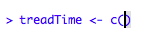
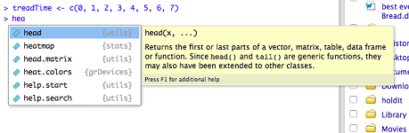
We get as far as typing
treadTime <– c(
| Figure 13 |
|
We just keep typing in our command until it is completed, as shown in Figure 14.
| Figure 14 |
|
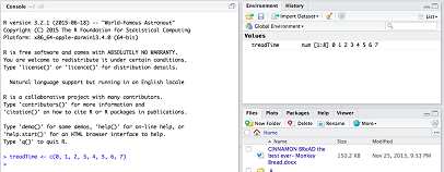
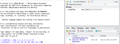
At that point we press the Enter key to tell R to perform the command. The result is shown in Figure 15. Notice that the only thing that happens in the left pane is that we get another prompt, the > sign. However, the top right pane now shows us that we have a variable, named treadTime, and that variable has the indicated values. This confirmation and display of the entities and their values that now exist in our R session is extremely useful.
| Figure 15 |
|
We will continue by typing the command
heartRate <– c( 73, 81, 88, 92, 98, 104, 111, 114)
| Figure 16 |
|
We type one more letter and the "helpful" display changes, as in Figure 17.
| Figure 17 |
|
Adding the fourth letter changes the display again, as in Figure 18.
| Figure 18 |
|
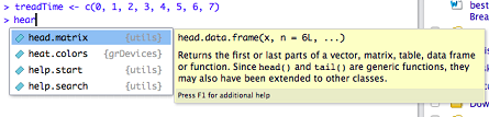
By the time we have typed "heart" the display has shrunk to that shown in Figure 19.
| Figure 19 |
|
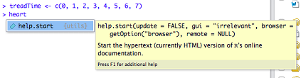
By the time we finish typing the entire command, the RStudio window should appear pretty much as is shown in Figure 20. We have yet to hit the "Enter" key so nothing else has happened.
| Figure 20 |
|
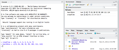
To get to Figure 21 we hit the "Enter" key to tell R to perform the command. R did not find a problem with our requested action so it performed it. RStudio, which monitors R confirms this by displaying the new variable, heartRate, and its initial values in the top right pane.
| Figure 21 |
|
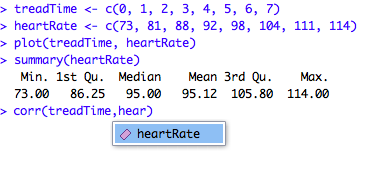
We can show off a little bit by asking R to create a scatter plot of the treadTime values against the heartRate values. To do this we just type
plot(treadTime, heartRate)
| Figure 22 |
|
How about another R command:
summary(heartRate)
   Min. 1st Qu.  Median    Mean 3rd Qu.    Max.
  73.00   86.25   95.00   95.12  105.80  114.00
Thus, in one simple command we learn the minimum value, 73, the maximum value, 114, the median (or middle) value, 95, the mean (numerical average) value, 95.12, the first quartile (25th percentile) value, 86.25, and the third quartile (75th percentile) value, 105.8.
| Figure 23 |
|
Figure 23 concludes with an attempt to submit another command. In the process of typing this command, in the middle of typing heartRate, the system is offering "heartRate" as a suggestion to complete the typing. To accept that offer, we just need to press the "Enter" key. That will take us to Figure 24.
A careful observer will notice that the "vertical insertion bar" is missing in that last line of Figure 23. It really is not so much missing as it was not captured when the screen image was taken. The vertical bar "flashes" and if it is not present when the image is captured then it will not be in the image. That is what happened in Figure 23. There really was a vertical bar between the "r" and the ")" in that line, and you would see it flashing if you did this on your machine.
| Figure 24 |

|
There are a few ways we can finish entering the command seen at the bottom of Figure 24. First, we could type the right parenthesis. RStudio knows that it supplied the right parenthesis already displayed in Figure 24, so our new right parenthesis will just replace that one. second, we could use the cursor controls or the mouse to move the insertion point beyond the right parenthesis. In either of those two cases our next action would be to press the "Enter" key. Our third option would be to just press the "Enter" key. RStudio would just assume that we wanted to complete the command with the right parenthesis that it supplied.
Use any of those methods to complete the command and ask R to execute it.
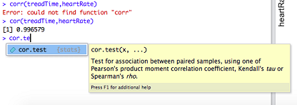
The first line of Figure 25 is the command we entered.
The second line of Figure 25 is the error message that R gave to us because the line we entered was incorrect. There is no predefined function called "corr" in R. Getting an error message like this is actually quite common. It just means that we have to fix what we entered.
The correct line
cor(treadTime,heartRate)
| Figure 25 |
|
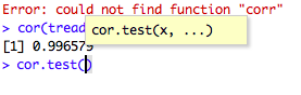
We conclude Figure 25 by starting to type the command
cor.test(treadTime,heartRate)
| Figure 26 |
|
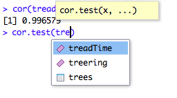
Then, as we start to type "treadTime" RStudio again offers to complete our work, suggesting "treadTime". Again, press the "Enter" key to accept that offer.
| Figure 27 |
|
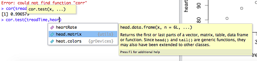
Figure 28 shows that RStudio has filled in "treadTime", and we have continued with ",hear", at which point RStudio is again trying to help by suggesting three things. In Figure 28 the second option is highlighted. We want the first so we could click on that, or we can just keep typing away ourselves.
| Figure 28 |
|
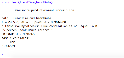
Either way, we finish the command and press the "Enter" key. This produced the multi-line output shown in Figure 29. Here we have lots of answers generated by our one simple command.
| Figure 29 |
|
You may notice that the last three lines of the output shown in Figure 29 give exactly the same simple answer that we got earlier from the "cor" function in Figure 25.
| Figure 30 |
|
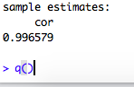
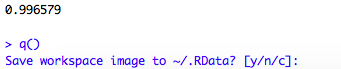
We conclude Figure 30 with the "q()" command to ask R to quit. R responds by asking if we want to "Save workspace image to"? We can respond to this by typing "y" for "yes", "n" for "no", or "c" for "cancel the quit request".
Remembering that this web page is just meant to demonstrate some of the features of R and of RStudio, we will respond with "y" to cause the program to quit but to save the workspace.
| Figure 31 |
|
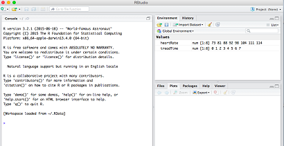
Saving the workspace means that we can restart R or restart it through RStudio, and it will pick up right where we left off. Let us try that. We will restart RStudio using the same method we did back between Figure 8 and Figure 9.
| Figure 32 |
|
There are two things to notice in Figure 32. First, toward the bottom of the "splash screen" shown in the left pane, R is telling us that
(Workspace loaded from ~/.RData). Second, in the upper right pane we see that the two variables that we had created before, namely,
treadTimeand
heartRatehave been restored. Thus, we could pick up our work right where we left off.
©Roger M. Palay
Saline, MI 48176 August, 2015