RStudio — Mac Install and More

This page is based on the installation of RStudio on a Mac computer using the Firefox web browser. The process took place on August 22, 2016. The standard version of RStudio at that time was 0.99.903. Please understand that web pages change, software changes, and installation systems change. Thus, what is recorded here, although true at the moment of recording, may have changed by the time you read this.

Also, as I hope is obvious, the some of the images below have been annotated, in GREEN, to show you where you need to point and click.

Just a few quick notes:

Figures 5 and 6 only show up the first time you run RStudio on particular Mac.
Figure 7 is an annoying option that will come up each time you start RStudio on a Mac until you give in and finally Install this feature. It does not hurt to do so, but we will not be using it. If time permits I will create a new page to step through that installation.
The Figures 8 and beyond walk through a small demonstration of why we want to use an IDE (Integrated Development Environment) such as RStudio.
Many of the Figures have been shrunk to facilitate display and printing. This does compromise the readability of the images, but the images are really just there to verify and explain what you should be seeing on your screen. On a Mac you can see the actual image by pointing to the shrunken image, holding down the Option key and then click on the image.
This material has not been formatted for printing so if you do print it you will get a lot of blank space and the Figure numbers may be separated from the images by page breaks.
Most important, I am not a Mac user. Threfore, although the steps shown here work there may be shorter, more efficient ways to accomplish the same thing. Feel free to use any such shortcut open to you.

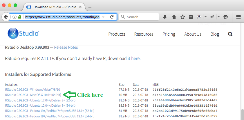
To install RStudio, we will go to the RStudio web site at the https://www.rstudio.com/products/rstudio/download3/#download/ web site. This should open a page which should appear as shown in Figure 1. Then in the list on the left locate the Mac OS X 10.6+ (64-bit) item and click on it.

Figure 1

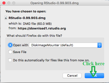
That will cause the file to download to your computer, after which the following screen should appear. Accept the default setting and just click on the OK button.

Figure 2

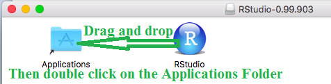
That will bring up a screen similar to that shown in Figure 3. Click and hold on the RStudio icon and drag it to the Applications folder on the screen.

Figure 3

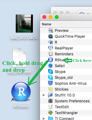
Once you have done the "drag and drop", double click on the Applications folder to open the screen shown in Figure 4. [You could also to this via the Finder application.]

We could open RStudio by clicking on the RStudio entry in the Applications window. Alternatively, we could click and hold the mouse key on the RStudio entry in the Applications window and then drag that item to the desktop and drop it there. This second approach has been done in Figure 4, giving us a RStudio icon on the desktop. Then, to start RStudio we merely need to double click on the RStudio desktop icon. Either way, at this point we want to start RStudio.

Figure 4

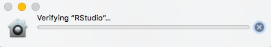
The small screen shown in Figure 5 should show up and then disappear. This should only happen the first time you start RStudio.

Figure 5

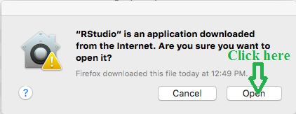
After that you should get another screen, shown in Figure 6, that only shows up the first time you run RStudio. For this screen you click on the Open button to move forward.

Figure 6

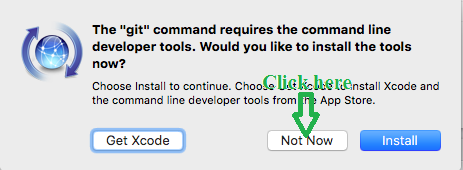
The next screen is new to this version of RStudio. It allows you to install some extra features, features that we will not be using. Since we will not use them, you can click on the Not Now button. However, at some point you will probably want to install the extra features if for no other reason that you will have decided that you do not want to see this screen again because it will show up each time you start RStudio.

Figure 7

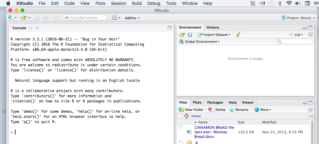
RStudio starts with a screen similar to that shown in Figure 8. There are three panes in this window, the Console, the Environment (which has a History tab), and the File (which also has tabs for Plots, Packages, Help, and Viewer) panes.

The Console pane is really an R session. What you see is the splash screen from the start of R.

Figure 8

As long as we have started RStudio we might as well try it out. We have the following problem. Walking around near the parking lot I found and collected 8 stones. I then weighed those stones and obtained the following measurements.

Weight of the stones I found
4.7	6.9	5.2	5.7	4.8	5.3	6.4	5.1

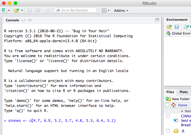
We want to put those values into RStudio. To do this, in the Console pane, we enter the command
stones <- c(4.7, 6.9, 5.2, 5.7, 4.8, 5.3, 6.4, 5.1)
in the Console after the > prompt.. This produces the image shown in Figure 9.

Figure 9

Now, to have R perform the command, we hit the Enter key on the keyboard. The result is shown in Figure 10.

Figure 10

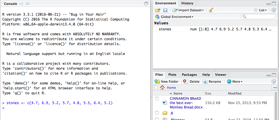
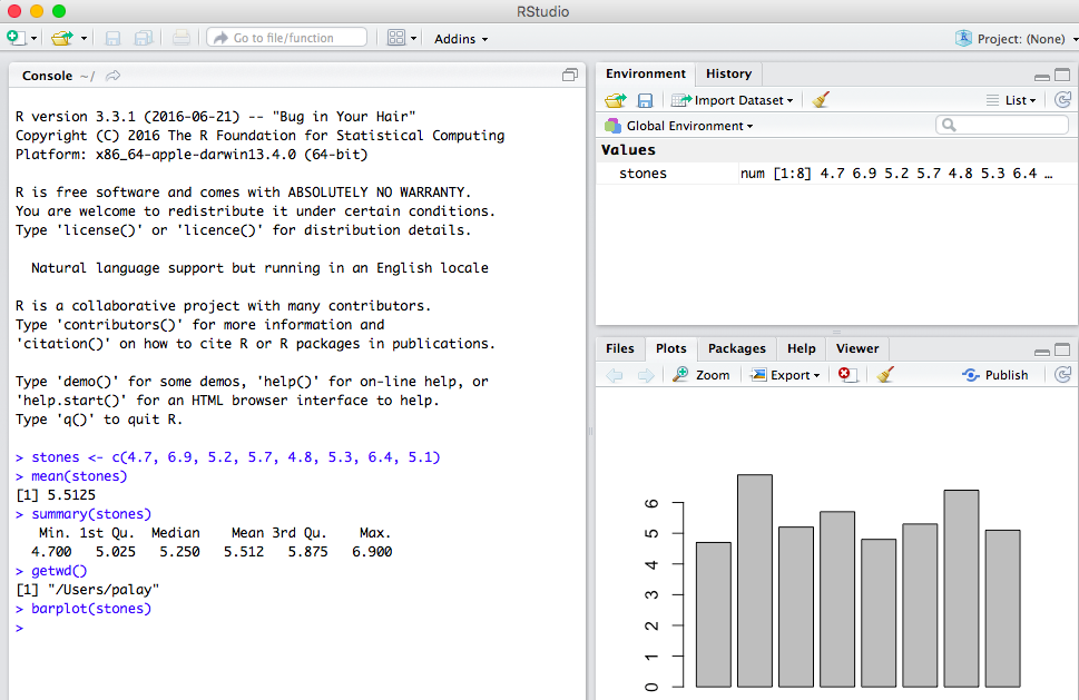
Our command has caused R to create a variable called stones, and to assign that variable the list of values that we specified. The Environment pane monitors the variables that have been defined. It also displays the first values stored in those variables. We only have the one variable so far, but we can see it, the fact that it is num meaning numeric, that it has eight values in it (items 1 through 8), and the value of the first few of those items.

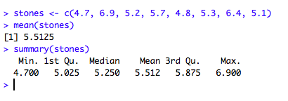
Let us do two more operations on the data. First we will ask R to find the mean (the average of the values, i.e., add up the values and divide by the number of values), and second, we will get a summary of the values. The first command is
mean(stones)
which we enter and then press the Enter key. R responds with the value 5.5125. The second command is
summary(stones)
which produces six values: the lowest value in the data, the 1^st quartile, the median value, the mean value, the 3^rd quartile, and the largest value in the data. You might note that R gives these with only 3 decimal places whereas R gave the mean value with 4 decimal places.

Figure 11

A completely different kind of command is getwd() shown in Figure 12. That command is a function that retrieves the working directory that R and RStudio are using at that time.

Figure 12

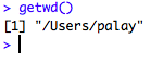
The result of using the command is C:/Users/palay, indicating that as the location of any files that we are using or that we might want to save. More on that later.

We can demonstrate yet another type of command, namely,
barplot(stones)
shown in Figure 32. The result of that command is a new plot, shown in the lower right pane, that is a bar plot of the data held in the variable stones.

Figure 13

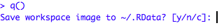
Finally, we use the q() command to tell R and RStudio to quit. For Figure 14 we have typed the q() command and pressed the Enter key. R then asks us if it should save the "workspace". This is also shown in Figure 14.

Figure 14

We want to save the workspace, so we answer "y", as shown in Figure 15.

Figure 15

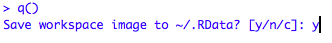
Once we press the Enter key R session will stop and the RStudio will close.

By "saving the workspace" we have told R to save all of our variables in a "hidden" file called .RData, and to save that file in the "working directory". We can see this if we open RStudio again (by double clicking on the RStudio icon on the desktop). We have done this to generate Figure 16.

Figure 16

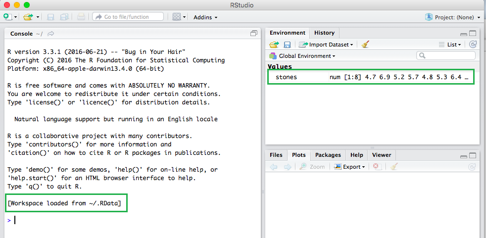
Two things to note in Figure 16 are the new last line of the "splash" screen from R telling us that the workspace has been loaded from the file and the fact that the one variable we had in our previous session is still defined. Both of those items have been highighted in Figure 16.

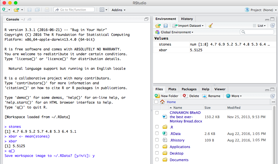
In fact, if we click on the Files tab in the lower right pane we change the display to that shown in Figure 17. In that pane we can see that the file .RData is now in that directory, that the file size is 2.6KB, and that it was created on Aug. 22 at 1:05 PM. In fact, a new history file called .Rhistory was created at that same time, the moment when we closed our previous session.

We will finish this introduction with a few more commands also shown in Figure 17 along with the resulting output from R. First, the command stones causes R to display the contents of the variable stones. Then the command
xbar <- mean(stones)
has R compute the mean and then store that value in the new variable xbar. Note that R does not display the value of xbar at that time, although RStudio displays it in the Environment pane. Then the command xbar causes R to display the value stored in the variable. Finally, the command q() causes R to ask if it should save the workspace. Again we respond with y. Once we press the Enter key the program will save the workspace and close.

Figure 17

At this point we will shift gears and look at the preferred, and expected, method of opening a new RStudio session. To do this we will plug in the USB thumb drive given out in class. When I did this on my computer the computer response was to display the icon shown in Figure 18 on the desktop. contents of the USB drive.

Figure 18

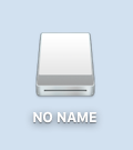
If we double click on the image of Figure 18 we get Figure 19 which displays the contents of the thumb drive. (You may need to look at Figure 20 to see a different form for displaying the contents of the drive. Different setting on different computers may cause either Figure 19 or Figure 20 to show up first.)

Figure 19

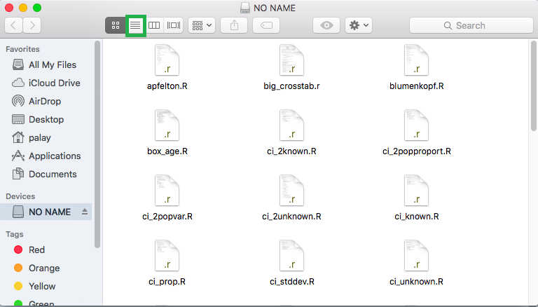
As noted above, there are other ways to display the contents of the drive. If you had the display in Figure 19 you can switch to the display in Figure 20 by clicking on the

icon, highlighted in Figure 19.

Figure 20

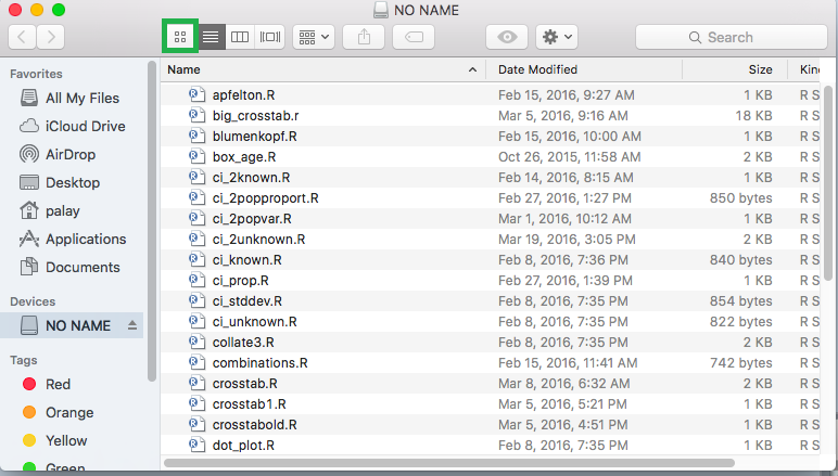
If you have the display shown in Figure 20, you can switch to the display shown in Figure 19 by clicking the

icon, highlighted in Figure 20.

We want to start from the display shown in Figure 19. Using that as a starting point, place the mouse over an open area and right click (or hold down the Control key and click the mouse pad or the one-button Mac mouse). That should bring up the small window shown in Figure 21.

Click on the New Folder option. This will produce an icon for that new folder as shown in Figure 22.

Figure 21

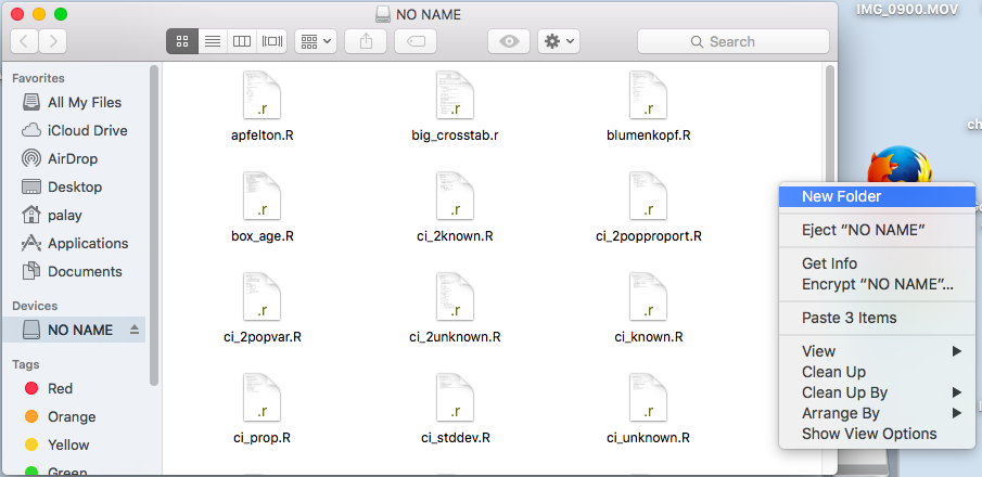
Figure 22

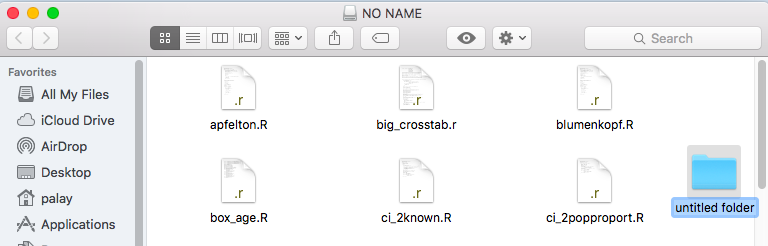
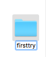
We can change the name of the New Folder from untitled folder to any name of our choice. In Figure 23 I have changed the name to firsttry.

Figure 23

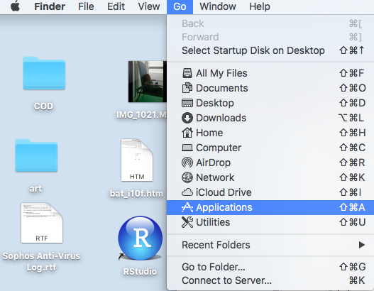
Our next goal is to create a file, in our new folder, and we ant that file to be associated with RStudio. To do this we will use the TextEdit program. To start that program we return to the Applications window. Figure 24 shows, again, the Finder window. In there we select, click on Applications.

Figure 24

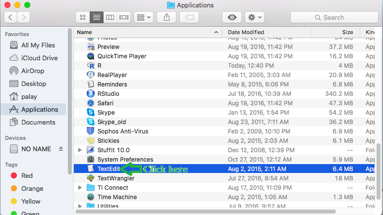
In the Applications shown in Figure 25 we find and select, click on, the TextEdit program.

Figure 25

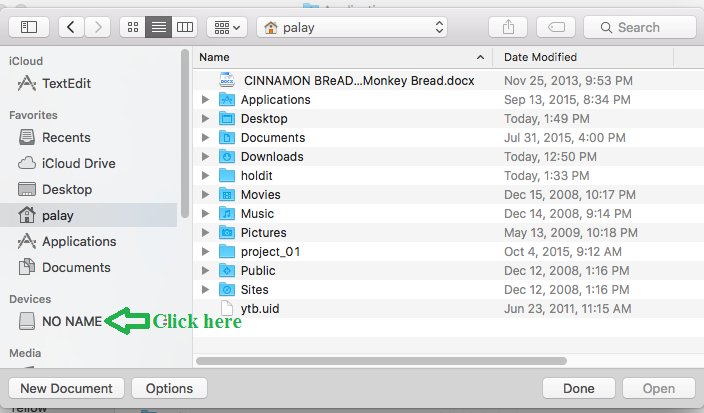
TextEdit starts and gives us a screen that will let us open an existing file, look around in different drives and folders, or create a new file (new document). We want to have our fie exist on the thumb drive. Therefore, click on the No Name item at the left of the screen.

Figure 26

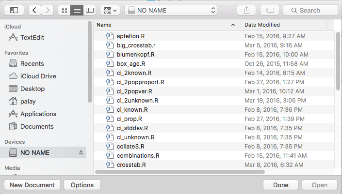
This will change the display to show the items, the files and folders, that are on the the thumb drive. The list appears in Figure 27.

Figure 27

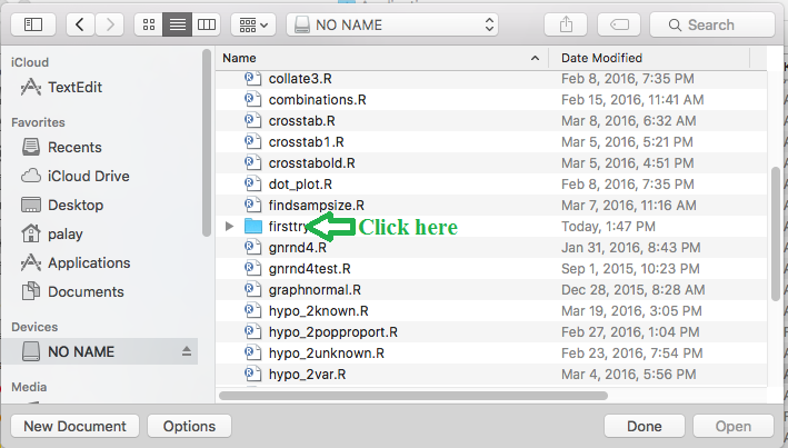
We do not want to add a new file here. Rather, we want to add a new file in the folder, firsttry, that we created earlier. firsttry does not appear in Figure 27, but we can scroll down the display to reveal firsttry, as shown in Figure 28.

Figure 28

From there we can click on firsttry to show all the files and folders that are in that directory.

Figure 29

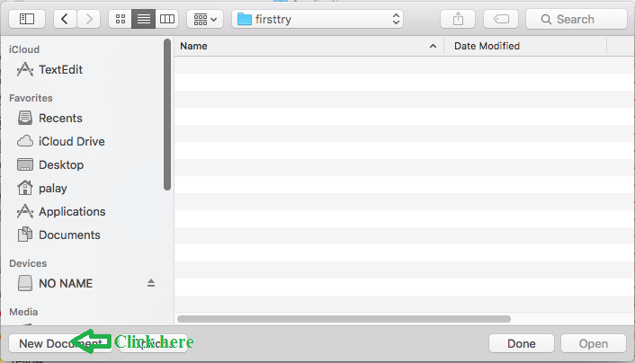
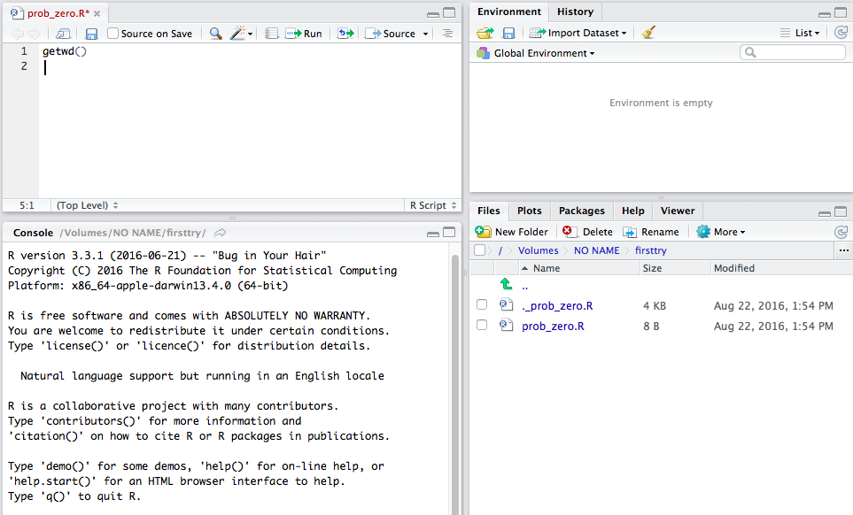
As we expect, having just created the folder, we find that there is nothing in it. We want to create a new file here so we click on the New Document button. This opens a blank document in the editor as shown in Figure 30.

Figure 30

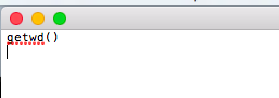
The only thing we want to add here is the command getwd(). We type that into the document ending up with the image shown in Figure 31.

Figure 31

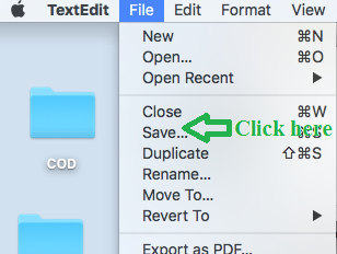
To save the document we click on the File option in the menu bar and then select the Save... option from the dropdown window.

Figure 32

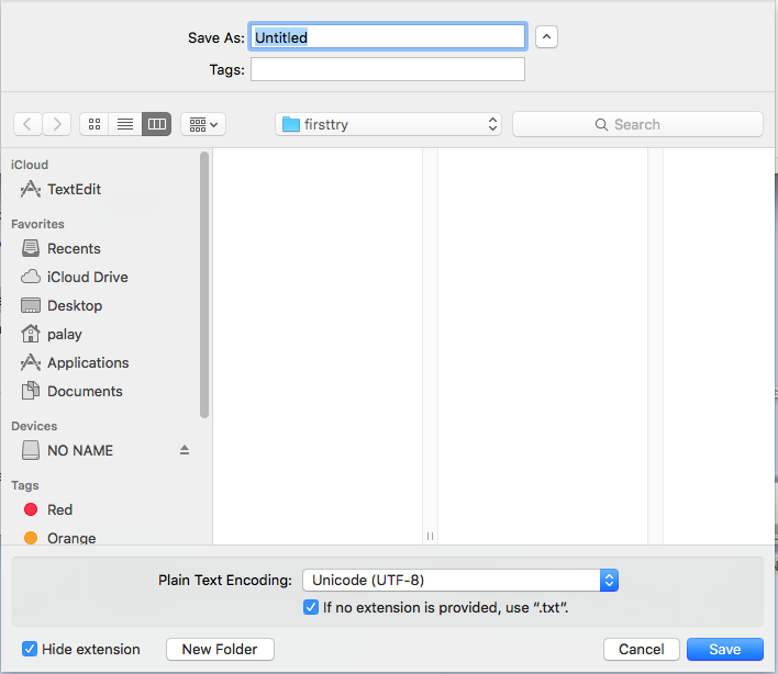
This brings up the screen shown in Figure 33. This will not only display the exisiting files and folders in our current location (remember that there are none since we just created the folder) but also allow us to save the file as a new file. The system proposes a title, in this case untitled in the box toward the top of the screen.

Figure 33

We will replace that proposed title by our own, in this case prob_zero.R, as shown in Figure 34.

Figure 34

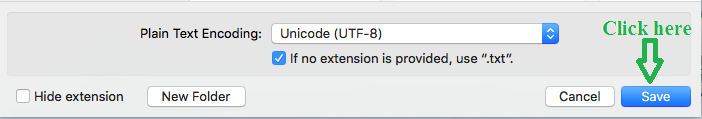
Once that is done we move to the bottom of the screen and click on the save button.

Figure 35

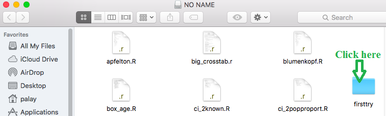
We are done with TextEdit. If we return to our screen as we left it in Figure 23, we could now click on our folder, firsttry, to display the conents of that foldeer.

Figure 36

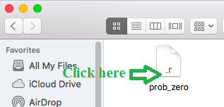
In Figure 37 we see that we have just one file, named prob_zero, and that it is of type .r.

After all of this work we can finally see the beauty of our actions. We double click on the file icon and the system will open RStudio. Not ony will it open RStudio, it will also set the working directory to be our folder and it will load the file we created, prob_zero.R, into the editor (which now shows up as a fourth pane in the RStudio window).

Figure 37

You might note, in Figure 38, that since this is our first time starting RStudio from this folder the R program did not have any workspace to recover, and therefore, there is no message at the end of the splash screen about loading a workspace.

Having a file into which we can type commands and then, as we will see, execute those commands is a significant advantage. Among other things, it allows us to take our work to another computer, to share our work with others, and to record and publish our work. This is an essential skill that all statisticians need to have.

Figure 38

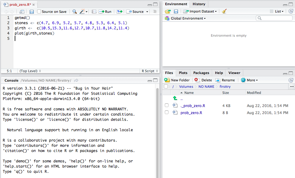
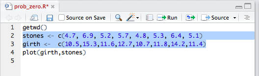
To demonstrate this, in the editor pane, type the following commands

getwd()
stones <- c(4.7, 6.9, 5.2, 5.7, 4.8, 5.3, 6.4, 5.1)
girth <-  c(10.5,15.3,11.6,12.7,10.7,11.8,14.2,11.4)
plot(girth,stones)

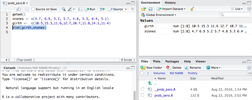
Actually, if you have this page open and you have your RStudio session open as shown in Figure 38, you can just highlight the commands above, copy them via the open Apple-c key sequence, click on the editor pane, and paste the commands via the open Apple-v key sequence. This saves a lot of typing. Your editor pane should appear as in Figure 39.

Figure 39

Now that we have the commands in the editor, we can execute any of them by highlighting the command and then clicking on the

icon in the editor pane.

Figure 40

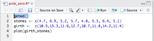
In Figure 40 the getwd() command was highlighted. If we then click on the

icon RStudio responds with Figure 41.

Figure 41

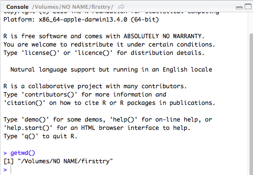
Remember that getwd() produces the name of the current working directory. In Figure 41 we see that it is exactly what we expected, we are in the firsttry folder in the NO NAME drive.

Now we can highlight the next two commands, as shown in Figure 42.

Figure 42

If we again click on the

icon RStudio copies those commands to the Console and executes them. The result is seen in Figure 43.

Figure 43

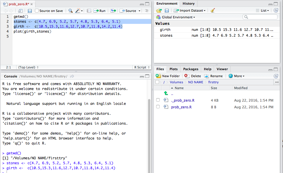
In Figure 43 we note that the commands have been performed, though they do not produce any output. We see in the Environment pane that the two variables have indeedd been defined.

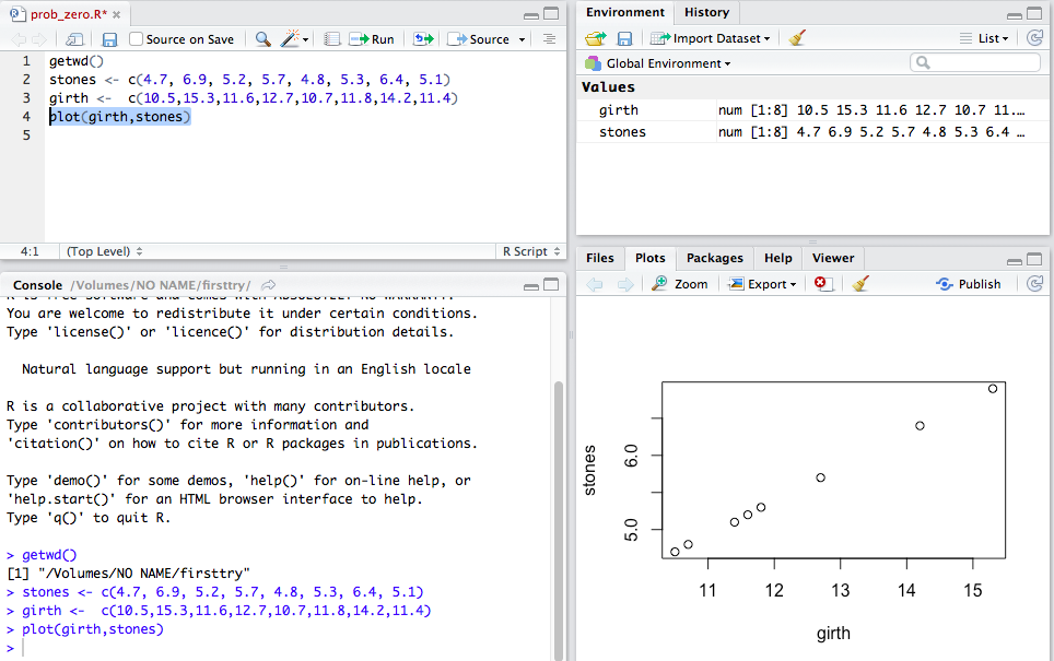
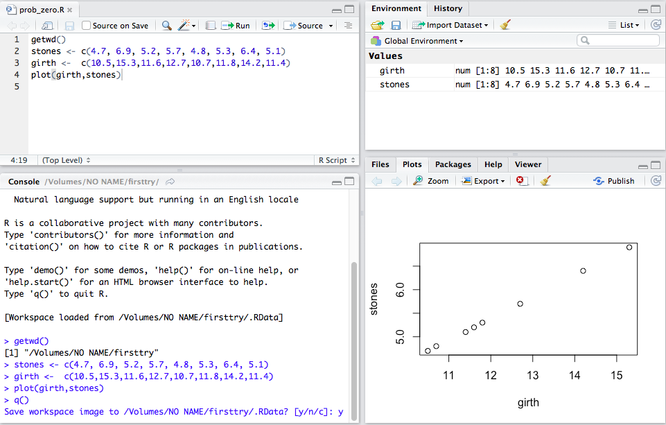
Now we hghlight the last command and then click on the

icon to get the screen shown in Figure 44.

Figure 44

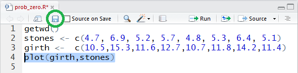
At this point we should note that we made changes in the editor version of our file, but we have not saved those changes back to the file. To save the file as it apears in the editor pane we click on the

icon as highlighted in Figure 45.

Figure 45

We can tell that this has worked by looking at the Files tab in the lower right pane. In Figure 46 we see that pane and we note that the size and date/time stamp for the file have changed.

Figure 46

Of course we can open the Plots tab and still see our beautifu scatter plot. And we are free to just type a command into the Console, such as the q() command to end the session. As usual, R responds by asking if the workspace should be saved. We respond y; press the Enter, and our RStudio session ends.

Figure 47

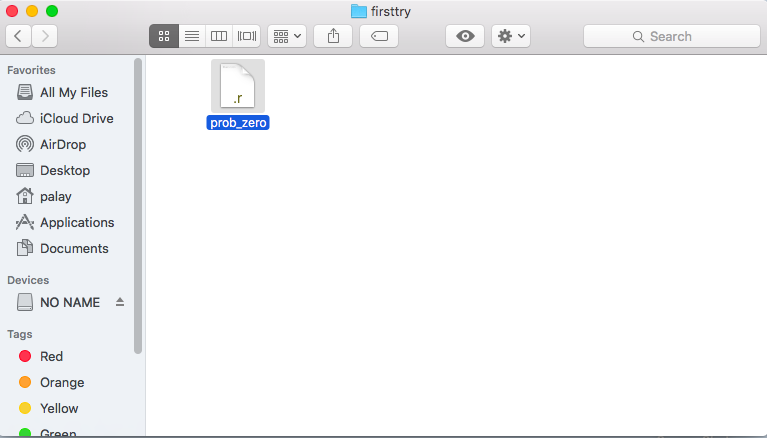
It is interesting and important to note the file that shows up in our Finder window for the firsttry foldere. It is shown in Figure 48. We note that only one file seems to be in the folder.

Figure 48

This is an unfortunate "feature" of the Mac operating system. By default, "hidden files" do not show up in the Finder view of a folder's contents. We actually have three "hidden files" in this folder. To see that we have those files we will just double click on the file name to open a new RStudio session, shown in Figure 49.

Figure 49

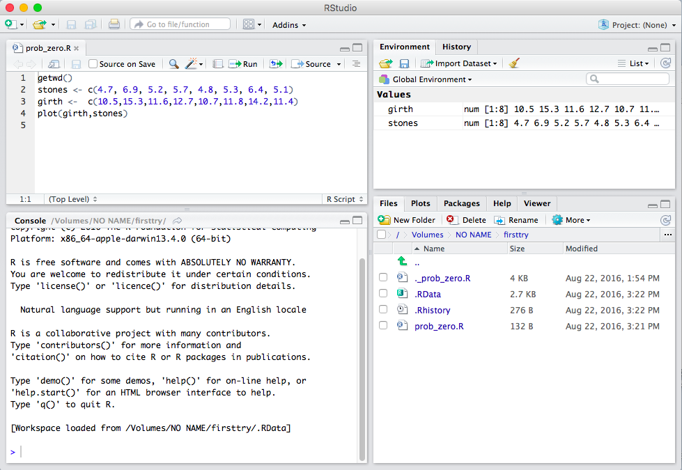
In the Files tab in the lower right pane we see all the files that are in the folder. Of particular importance are the two files .RData and .Rhistory, the first holds the variables that we have defined, anfd their contents, while the second holds the list of commands that we have given.

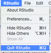
With nothing else to do now we can close the session. In this case we will do so by clicking on the RStudio item in the menu bar and then clicking on the Quit RStudio option.

Figure 50

One last task is for us to see how we can safely remove the USB drive. On a Mac we can do this by right clicking (or hold down the Control key and do either a mouse pad click or a one button mouse click) to get the small window shown in Figure 51.

Figure 51

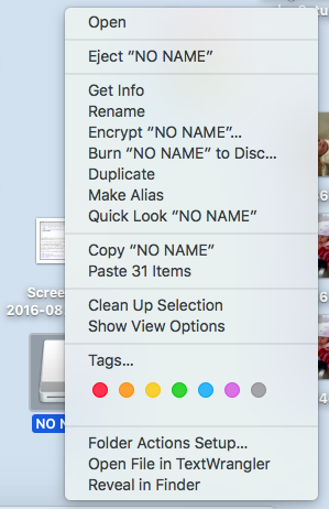
In that list of actions we select Eject "NO NAME". If there are no open files on the USB drive then the operating system will effetively disconnect the USB drive and we are free to remove it.

Return to Software Installation