Computing in R: Frequency Tables -- Grouped Values

Please note that at the end of this page there is a listing of the R commands that were used to generate the output shown in the various figures on this page.

This page presents R commands related to building and interpreting frequency tables for grouped values. To do this we need some example data. We will use the values given in Table 1.
Because this data has so many different values, it would not make sense to look at it as discrete values. Rather, we want to group these values into bins or buckets. In the preceding discussion of grouped data page we developed a table such as Table 2 to give the appropriate values for this data.

Table 2 has been created within this web page, based on the values displayed in Table 1. Our task is to find the commands that we can use in R to generate this same table.

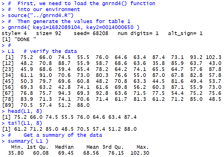
To start, we need to generate the data in R and then find the low and high values in that data. Figure 1 shows the gnrnd4() statement used to generate the same data in R, followed by the L1 statement so that we can be sure that we generated the right data. A quick comparison shows that the values are identical. Figure 1 also demonstrates the use of the head() and tail() functions as a shorter way to verify the data. We follow that with the summary(L1) statement. Figure 1 shows the related output, including a display of the minimum and maximum values.

Figure 1

We need those values so that we can make a decision about the places where we want to break the range of values, from a minimum of 35.8 to a maximum of 102.3. In order to have some nice "endpoints" to our intervals we can start them at 30, end them at 110, and have an interval width of 10. There is no real need to put those values into variables, but we can do just that. The first 3 statements in Figure 2 make such assignments.

Figure 2

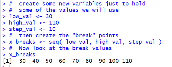
The seventh line in Figure 2, x_breaks <- seq( low_val, high_val, step_val) creates a new variable and stores in that variable the sequence of values 30, 40, 50, 60, 70, 80, 90, 100, and 110. We see those values displayed as a result of the command x_breaks.

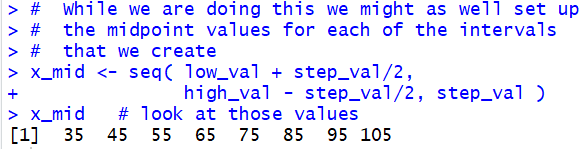
As long as we are using the seq() function, we might as well set up a sequence of the midpoint values. Figure 3 shows the command that we use, namely, x_mid <- seq( low_val+step_val/2, high_val-step_val/2, step_val), to create such a sequence, and that same figure shows the values stored in x_mid.

Figure 3

R has a command, cut(), that expects us to give it a collection of values and the break points to use with those values. We formulate the command as x <-cut(L1, breaks=x_breaks), as shown in Figure 4.

The result of the cut() command is a collection of intervals, all conforming to the break points that we gave cut() with the specific interval values representing the interval into which the corresponding value in the data, in our case L1, falls. Consider the output shown in Figure 4.

Figure 4

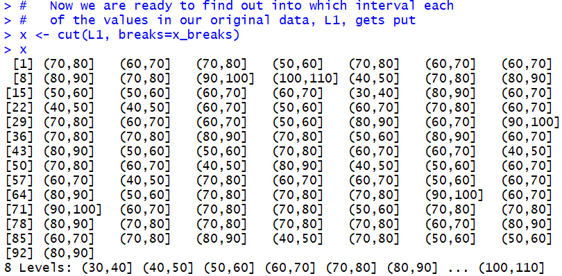
The first value in L1, the first value in Table 1, is 75.2. That value falls into the (70,80] interval. Therefore, the first value out of cut() is (70,80]. The second value in L1 is 66.0; that value falls into the (60,70] interval. Therefore, the second value out of cut() is (60,70]. The third value in L1 is 74.5; that value falls into the (70,80] interval. Therefore, the third value out of cut() is (70,80]. The fourth value in L1 is 55.5; that value falls into the (50,60] interval. Therefore, the fourth value out of cut() is (50,60]. And so on through the rest of the values in L1.

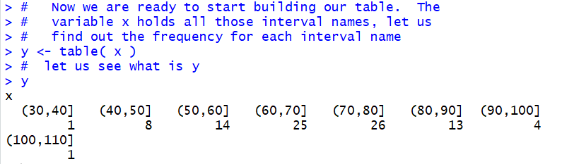
The interesting thing here is that we start with L1 as a collection of values and we end up with x holding a collection of interval specifications. This means, that if we want to know how many of the values in L1 fall into the interval (80,90] we just need to find the number of (80,90] entries in x. We should notice, at this point, that x is really a collection of discrete values. Therefore we can return to the things we learned in dealing with discrete value, namely the use of the table() function, to get the frequency of each of the discrete values. The command y <- table( x ) has R computing those frequencies and storing the result in the valiable y.

Figure 5

Then, just as we did for the discrete case, we form a data frame based on the values in our discrete variable y.

Figure 6

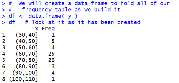
The display of our data frame, given in Figure 6, has the same values as we had in the first two columns of our goal table shown back in Table 2. What remains to be done is to compute the remaining columns and attach them to the data frame.

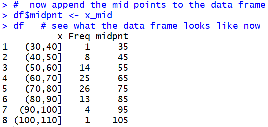
We start that process by adding the midpoint values that we have already computed. The statement df$midpnt <- x_mid appends those values as a new column in the data frame, and it titles that column as midpnt. The result is shown in Figure 7.

Figure 7

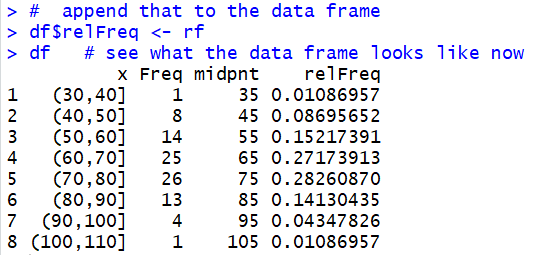
We continue the process by computing the relative frequency. Recall that the relative frequency is the result of dividing each of the particular frequencies by the number of values in the original table. The command shown in Figure 8, rf <- df$Freq/sum(df$Freq), finds the number of values in the table by finding the sum of all the frequencies.

Figure 8

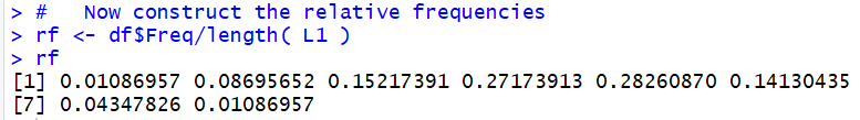
Comparing the values displayed in Figure 8 with those in the fourth column of Table 2 confirms our calculation. We just have to append those values to our data frame. This is done in Figure 9.

Figure 9

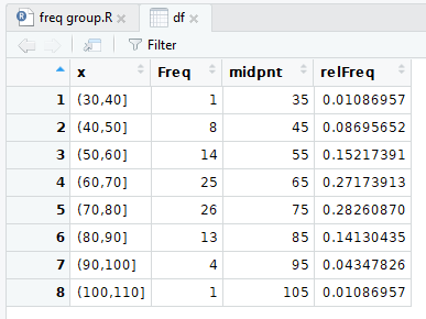
We can use the View(df) command to display, in the top left pane within the RStudio window, pretty view of the data frame. The command is shown in Figure 9.5.

Figure 9.5

And the pretty display is shown in Figure 10.

Figure 10

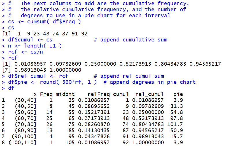
We continue the process by computing the cumulative frequency, the relative cumulative frequency (which is mathematically identical to the cumulative relative frequency), and the number of degrees in a pie chart that should be allocated to this group (assuming that we want to make a pie chart which we know we should not do). Figure 11 shows the specific commands, and a final display of the data frame.

Figure 11

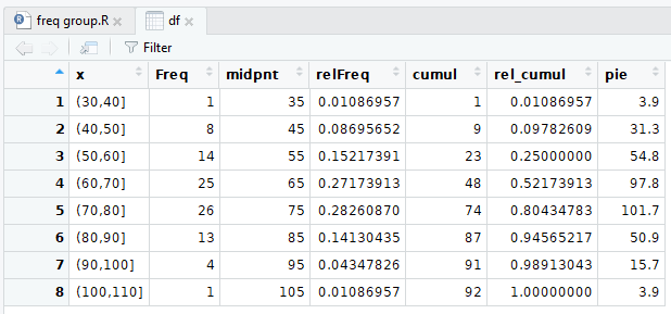
Also recall that as we change the data frame the system automatically updates the "view" of the data frame. Therefore, without having to perform another View(df) command in our RStudio session, the "pretty" view of the data frame now appears as in Figure 12.

Figure 12

To this point in the web page we have seen a sequence of steps in R that we can use to go from an initial problem statement to our desired solution. The process of those steps is to take a collection of data, determine how we can break the range of those values into equal width partitions, count the frequency of the original data values in each of the partitions, and form an expanded frequency table based on those frequencies. The steps shown above from Figure 1 through Figure 12 walk us through that process. We could study, memorize, transcribe those steps and then follow them whenever we have this kind of a problem.

Alternatively, as we did for discrete values, we could write a function that just captures those steps so that we can perform the steps by just calling the function. The function that we created for the discrete case was called make_freq_table() and it amounted to 22 lines of code, 9 of which were comments. The function we create for this task, the function collate3(), is a bit longer and more complex. It does follow the same pattern that we have just stepped through, but it also has a few small detours in it. Rather than explain the function in a step by step manner here, the listing of the function is provided both here and on another web page, the latter providing a discussion of the detailed structure and steps of the function. The link to that other page is Explanation of collate3.R. The listing of the function here is:

collate3 <- function( lcl_list, use_low=NULL, use_width=NULL, ...)
  { 
    ## This is a function that will mimic, to some extent, a program
    ## that we had on the TI-83/84 to put a list of values into
    ## bins and then compute the frequency, midpoint, relative frequency,
    ## cumulative frequency, cumulative relative frequency, and the
    ## number of degrees to allocate in a pie chart for each bin.
  
    ## One problem here is that getting interactive user input in R
    ## is a pain.  Therefore, if the use_low, and or use_width
    ## parameters are not specified, the function returns summary
    ## information and asks to be run again with the proper values
    ## specified.
  
   lcl_real_low <- min( lcl_list )
   lcl_real_high <- max( lcl_list ) 
   lcl_size <- length(lcl_list)
   
   if( is.null(use_low) | is.null(use_width) )
   {

     cat(c("The lowest value is ",lcl_real_low ,"\n"))
     cat(c("The highest value is ", lcl_real_high,"\n" ))
     suggested_width <- (lcl_real_high-lcl_real_low) / 10 
     cat(c("Suggested interval width is ", suggested_width,"\n" ))
     cat(c("Repeat command giving collate3( list, use_low=value, use_width=value)","\n"))
     cat("waiting...\n")
     return( "waiting..." )    
   }
  ## to get here we seem to have the right values
  use_num_bins <- floor( (lcl_real_high - use_low)/use_width)+1
  lcl_max <- use_low+use_width*use_num_bins
  lcl_breaks <- seq(use_low, lcl_max, use_width)
  lcl_mid<-seq(use_low+use_width/2, lcl_max-use_width/2, use_width)
  
  lcl_cuts<-cut(lcl_list, breaks=lcl_breaks, ...)
  lcl_freq <- table( lcl_cuts )
  lcl_df <- data.frame( lcl_freq )
  lcl_df$midpnt <- lcl_mid
  lcl_df$relfreq <- lcl_df$Freq/lcl_size
  lcl_df$cumulfreq <- cumsum( lcl_df$Freq )
  lcl_df$cumulrelfreq <- lcl_df$cumulfreq / lcl_size
  lcl_df$pie <- round( 360*lcl_df$relfreq, 1 )
  
  lcl_df
  }

If so desired, you could highlight that listing and copy it and then paste it to your own text editor, or even directly into an R or an RStudio session. Furthermore, a link to the actual function file is collate3.R.

To illustrate using the collate3() function we start with a source() command to load the function into our RStudio session. Then we just try to run the function to process the data that we still have in L1 using the collate3(L1) command. The result is shown in Figure 13.

Figure 13

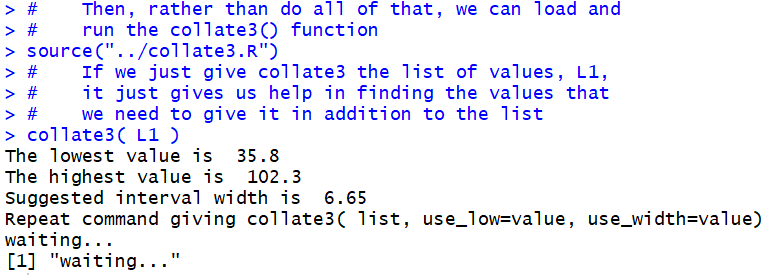
It turns out that collate3()really wants us to specify the starting point for our partitions and the width of the partitions. If we do not specify these, then collate3() assumes that we just do not know them, probably because we do not know the minimum and maximim values in the data. [Now, in this case we did know them. We found them back in Figure 1. However, we are trying to demonstrate using collate3() without relying on our previous knowledge.] In order to help us, collate3() does not just give up but, rather, it provides us with the minimum and maximum values, and it even suggests a width for the intervals.

We take that information and we reissue the command, this time as collate3( L1, 30, 10 ), telling the function to process the values in L1 and to construct partitions starting at 30 with a partition width of 10. This is shown in Figure 14.

Figure 14

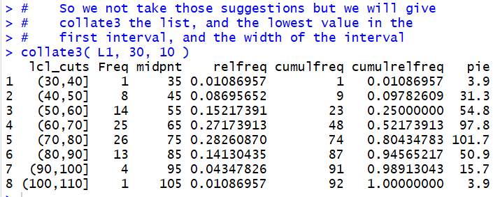
The result is the display of the data frame created by collate3(). In one step we accomplished all of the work that we went through in Figures 1 through 11 above.

It is worth doing this again but for different data values. The whole process, other than loading the functions, is shown in Figure 15.

Figure 15

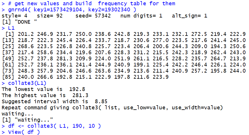
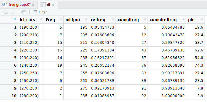
We use the command gnrnd4( key1=1573429104, key2=19302340 ) to generate all new data, the command L1 to display that data, the command collate3(L1) to find the minimum and maximum values, the command df <- collate3( L1, 190, 10) to create a data frame giving the expanded frequency table of the values in L1 based on partitions starting at 190 and having a width of 10, soring that data frame in the variable df, mand, finally, getting the "pretty" display of that data frame shown in Figure 16.

Figure 16

One feature that we have glossed over in this discussion is the decision to use intervals that are "closed on the right" as in a partition like (200,210]. In that partition, the value 210 would be part of the partition, but the value 200 would not. Instead, the value 200 is part of the partition (190,200].

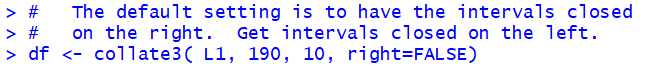
What if we want to use partitions that are "closed on the left"? To do this the change actually has to go back to the cut() statement, but rather than look there first, we note that colalte3() was written with this in mind. In order to have partitions that are closed on the left, you simply change the collate3() command to include the setting right=FALSE. We have an example of this in Figure 17 where we repeat our command with the new setting.

Figure 17

The result is reflected in the "pretty" display now shown in Figure 18.

Figure 18

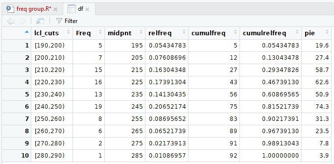
As you can see in Figure 18 we are now using partitions that are "closed on the left" an, as a result, the frequencies change in some of the partitions.

What has really happened here is that the setting "right=FALSE" was accepted by collate3() but passed on to the cut() function inside of the collate3() function. We can see how this setting changes the cut() function by looking at the statements and results in Figure 19.

Figure 19

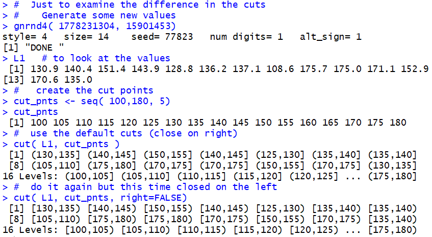
In Figure 19 we generate and display a new L1, this time with just 14 values. Note that the tenth value is 175.0 and the fourteenth value is 135.0. Then we generate a first version of the partition this time using the default "closed on the right" rule. Note that the tenth value here is (170,175] because that is where the tenth value in L1, 175.0, falls. The fourteenth interval (bin, bucket, group) is (130,135] because, when closed on the right, that is where 135.0 falls.

After that we generate a similar partition, but this time overriding that rule by setting right=FALSE. The new partition is "closed on the left". Note that tenth value here is [175,180) because, when closed on the left, that is where the tenth value in L1, 175.0, falls. The fourteenth interval (bin, bucket, group) is [135,140) because, when closed on the left, that is where 135.0 falls.

Here is the list of the commands used to generate the R output on this page:

# the commands used on Frequency Tables -- Grouped Values
#
#  First, we need to load the gnrnd4() function
#  into our environment
source("../gnrnd4.R")
#  Then generate the values for table 1
gnrnd4( key1=1682089104, key2=0014000650 )
#
L1   # verify the data
head(L1, 8)
tail(L1, 8)
#    Get a summary of the data
summary( L1 )
#  create some new variables just to hold
#  some of the values we will use
low_val <- 30
high_val <- 110
step_val <- 10
#  then create the "break" points
x_breaks <- seq( low_val, high_val, step_val )
#  Now look at the break values
x_breaks
#  While we are doing this we might as well set up 
#  the midpoint values for each of the intervals
#  that we create
x_mid <- seq( low_val + step_val/2,
              high_val - step_val/2, step_val )
x_mid   # look at those values
#
#   Now we are ready to find out into which interval each
#   of the values in our original data, L1, gets put
x <- cut(L1, breaks=x_breaks)
x
#
#   Now we are ready to start building our table.  The 
#   variable x holds all those interval names, let us 
#   find out the frequency for each interval name
y <- table( x )
#  let us see what is y
y
#  We will create a data frame to hold all of our 
#   frequency table as we build it
df <- data.frame( y )
df   # look at it as it has been created
#
#  now append the mid points to the data frame
df$midpnt <- x_mid 
df   # see what the data frame looks like now
#
#   Now construct the relative frequencies
rf <- df$Freq/length( L1 )
rf
#  append that to the data frame
df$relFreq <- rf
df   # see what the data frame looks like now
#   Let us look at the pretty version of the data frame
View( df )  #  note the capital V
#   The next columns to add are the cumulative frequency,
#   the relative cumulative frequency, and the number of
#   degrees to use in a pie chart for each interval
cs <- cumsum( df$Freq )
cs
df$cumul <- cs             # append cumulative sum
n <- length( L1 )
rcf <- cs/n
rcf
df$rel_cumul <- rcf        # append rel cumul sum
df$pie <- round( 360*rf, 1 )  # append degrees in pie chart
df
#
#    Then, rather than do all of that, we can load and 
#    run the collate3() function
source("../collate3.R")
#    If we just give collate3 the list of values, L1,
#    it just gives us help in finding the values that
#    we need to give it in addition to the list
collate3( L1 )
#    So we not take those suggestions but we will give
#    collate3 the list, and the lowest value in the 
#    first interval, and the width of the interval
collate3( L1, 30, 10 )
#
##############################
# get new values and build  frequency table for them
gnrnd4( key1=1573429104, key2=19302340 )
L1
collate3(L1)
df <- collate3( L1, 190, 10 )
View( df )
#   The default setting is to have the intervals closed
#   on the right.  Get intervals closed on the left.
df <- collate3( L1, 190, 10, right=FALSE)
##############################
#  Just to examine the difference in the cuts
#    Generate some new values
gnrnd4( 1778231304, 15901453)
L1   # to look at the values
#   create the cut points
cut_pnts <- seq( 100,180, 5)
cut_pnts
#  use the default cuts (close on right)
cut( L1, cut_pnts )
#  do it again but this time closed on the left
cut( L1, cut_pnts, right=FALSE)
#