Probability: Student's t
Return to Topics page
Introduction, Graphs, and Tables
An earlier page presented the Normal distribution.
It was symmetric,
continuous, bell-shaped, and based on a mathematical formula. Here we present
the Student's t distribution.
It too is symmetrical, continuous, bell-shaped,
and based on a mathematical formula.
The formulae are different, and the resulting "bells" are different,
but only slightly.
The big difference is that instead of having one
standard normal distribution we end up with a whole
class of slightly different standard Student's t distributions
where the different versions within the class are specified by
a new value, the degrees of freedom.
That is, there is one Student's t distribution for 2 degrees of freedom,
another for 3 degrees of freedom,
another for 4 degrees of freedom, and so on.
The lowest allowed degrees of freedom is 1.
For us, at this time, the degrees of freedom is always a whole number.
There is no limit on the highest number you can use. However, as we will see,
the higher the degrees of freedom the smaller the difference between a
Student's t and a Normal distribution.
We will start by looking at the graph of the density function for a
Student's t distribution with 2 degrees of freedom.
Figure 1 holds such a graph.
Figure 1
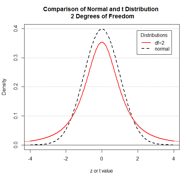
Remember that the normal distribution pictured here is the standard
normal distribution. It has mean=0 and standard deviation=1.
The same is true for the Student's t distribution. It has
mean=0 and standard deviation=1.
We certainly note the continuous,
symmetric, bell-shaped nature of both
distributions. However, the Student's t
distribution has shifted more of the
area under the curve toward the tails.
There is still 50% of the area to the left of 0,
but more of that area is further away from 0.
We were able to use a table to obtain the area to the left of any z-score
for the normal distribution.
For example, for that normal distribution
we could have looked at the following portion of the table to find
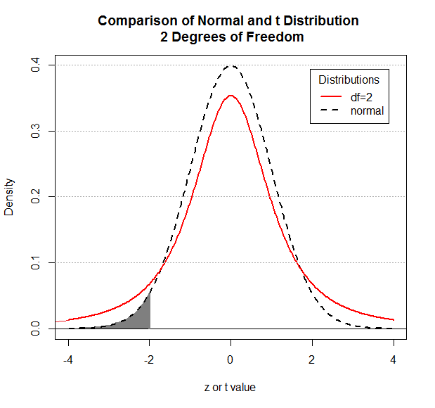
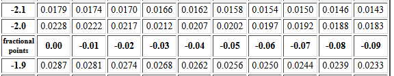 from which we would know that P(X < -2.00) = 0.0228.
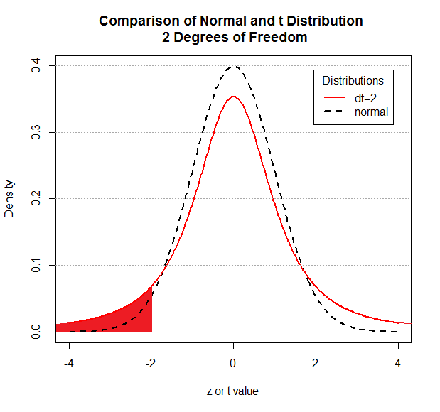
This is the area shaded in gray in Figure 2. The area under the
Student's t with 2 degrees of freedom
distribution and to the left of -2,
the area shaded in red in Figure 3, is clearly much larger.
from which we would know that P(X < -2.00) = 0.0228.
This is the area shaded in gray in Figure 2. The area under the
Student's t with 2 degrees of freedom
distribution and to the left of -2,
the area shaded in red in Figure 3, is clearly much larger.
Figure 2
|
Figure 3
|
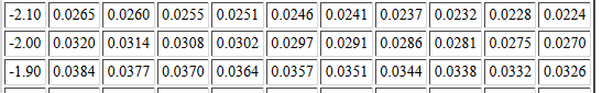
If we had a table for the standard Student's t
with 2 degrees of freedom,
then we would find the appropriate portion of the table
would look like that in Figure 4.
Figure 4: Portion of Student's t with 2 degrees of freedom
From that we can read that the P(X<-2.00) = 0.0918.
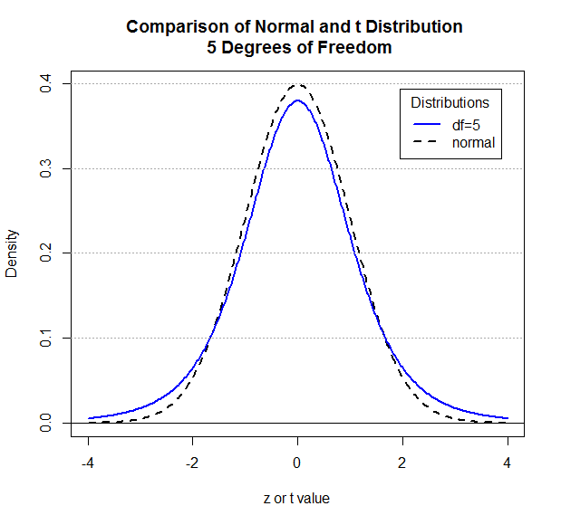
As noted above,
the higher the degrees of freedom the smaller the difference between a
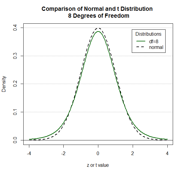
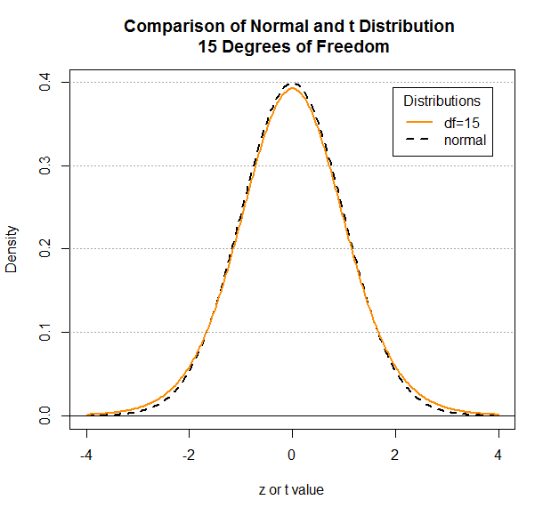
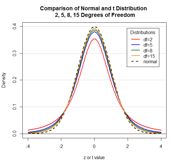
Student's t and a Normal distribution. The following figures
show the comparison between the normal distribution and the
Student's t with 5, then 8, then 15 degrees
of freedom, followed by a graph showing all putting all four
of the graphs together.
Figure 5
|
Figure 6
|
Figure 7
|
Figure 8
|
As you can see, by the time we get to 15 degrees of freedom
there is not much of a difference between the normal
and the Student's t distributions.
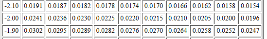
Were we to have a table for the Student's t at
15 degrees of freedom then the part of the table that includes
the t value -2.00 would be as shown in Figure 9
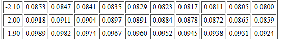
Figure 9: Portion of Student's t with 15 degrees of freedom
The values have changed, and they are getting closer to the values
in the normal distribution table.
The pattern of change continues as we increase the degrees of freedom.
Figure 10 shows 40 degrees of freedom.
Figure 10: Portion of Student's t with 40 degrees of freedom
Figure 11 shows 100 degrees of freedom.
Figure 11: Portion of Student's t with 100 degrees of freedom
The values in the tables always change as we increase the degrees of freedom and
they always move closer to the values in the normal distribution.
By the time we get to 40 degrees of freedom the difference
between the Student's t and normal values associated
with a t-score and z-score, respectively, is not seen until
the thousandths place. Really not much of a difference at all.
With different values for different degrees of freedom,
we would need a separate table for each degree of freedom.
To do this for the first forty possible degrees of freedom
in a textbook would take 40 pages. This is just not done.
Of course, we have no such page limit on the web. Here is a
link to an Index of Student's t tables
which serves as a gateway to tables for the first 100 degrees of freedom.
What, then, do books provide? They give a table of "critical values"
for the Student's t distribution. The authors have decided that
we will only be interested in knowing the t-value
that is associated with just a few probabilities. An example
of such a table can be found at
Critical Values of Student's t.
The start of the table is shown in Figure 12.
Figure 12
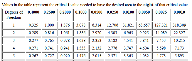
The first thing to notice about this table is that it gives t-scores
needed to have the specified area (the column heading) to the
right of that score for each of the degrees of freedom
(the row headings). The reason for looking right instead of left
is that this way we are dealing with positive t-scores, saving
printing all those negative signs.
This is not really a problem because the Student's t
is a symmetric distribution.
Therefore, although the table shows that for 5 degrees of freedom
we need a t-score of 3.365 to have just 0.0100 square units (1% of the area)
to the right of that value, we know that we would need a t-score of -3.365
to have 1% of the area to the left of that value.
The second thing to notice is that the table is useless
in finding P(X < 0.15) for 3 degrees of freedom.
We are only given columns for specified "critical" values, among which are
20% and 10%, but not 15%. Because we have the web tables noted above, we
would have no problem finding that probability there, but we cannot find it here.
If you ever wonder why so much research is reported
at the 0.05, or .01 level and not at the 0.03333
level, it is because the researchers had access to tables that had the 0.05
and 0.01 values, but not the 0.03333 values.
The third thing to notice about the table is that the row headings
increase by 1 degree of freedom for a while,
and then jump to steps of 10 degrees of freedom.
How could we use the table for 63 degrees of freedom?
We would just interpolate the values
between 60 and 70 degrees of freedom.
The fourth thing to notice about the table is that it
stops at 200 degrees of freedom. What do we do for 230 degrees of freedom?
We just say that with that many degrees of freedom there is so little difference
between the Student's t and the normal distributions that
we might as well use the normal table.
pt() in R
Of course, all this talk about tables has become almost historical.
We have functions in R to produce these values on demand.
The function pt() will give us the area under the curve to
the left of a specified t-score. We do, however, need to
give pt() both that t-score and
the number of degrees of freedom. For example, we could use the commands
pt(-2.0,2)
pt(-2.0,5)
pt(-2.0,8)
pt(-2.0,15)
to give us the very values that we so painfully
had to find in the four different tables on our web page.
Figure 13 shows the console record of those four commands
so that we can compare the results to those from the tables above.
Figure 13
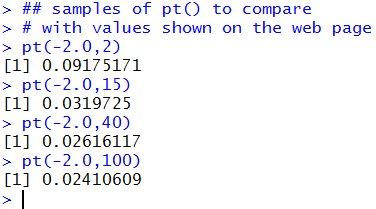
As usual, the R default is to display 7 significant digits.
There is no room in a book to display tables that show that many digits
and we really do not
need that many.
Unlike the table in a book (or the 100 web tables provided here), R
will also compute the area under the curve but to the right of a value.
To do this we add the lower.tail=FALSE argument to the command.
Consider the commands
pt(3.078,1,lower.tail=FALSE)
pt(2.353,3,lower.tail=FALSE)
pt(4.604,4,lower.tail=FALSE)
pt(3.365,5,lower.tail=FALSE)
shown in Figure 14.
Figure 14
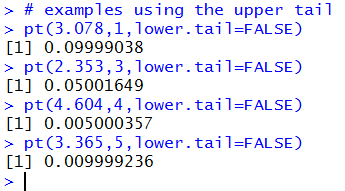
It is easy to believe that the pt() function worked, but we can actually
get a confirmation of that by looking back to Figure 12.
Each of the t-score and degree of freedom pairs in the pt()
statements in Figure 14 came from Figure 12. The results shown
in Figure 14, when rounded to 3 decimal places, are the
associated "critical value probabilities" of Figure 12,
namely, 0.10, 0.05, 0.005, and 0.01.
qt() in R
The qt() function in R accepts as arguments
a desired probability and the degrees of freedom.
The returned value of the function call
is the t-score needed for the specified degrees of freedom
in order to have the specified probability be the area
under that Student's t curve and to the
left of the t-score.
In a sense, the qt() function reads "backwards" from the
100+ big tables and "forwards" from the "Critical Values" table
with the understanding that the default for qt() is to look
"left" whereas the "Critical Values" table looks "right".
Consider the following examples:
qt(0.10,1)
qt(0.05,3)
qt(0.005,4)
qt(0.001,5)
These statements are shown in Figure 15.
Figure 15
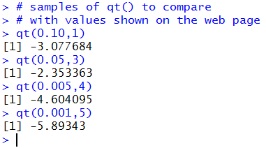
The results, the negatives of the values used in Figure 14,
are the expected values given that the
Student's t distribution is symmetric.
Fortunately, the lower.tail=FALSE argument
can be added to the function calls to
have qt() look to the "right".
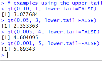
The same examples, with the added argument, would be
qt(0.10, 1, lower.tail=FALSE)
qt(0.05, 3, lower.tail=FALSE)
qt(0.005, 4, lower.tail=FALSE)
qt(0.001, 5, lower.tail=FALSE)
These statements are shown in Figure 16.
Figure 16
Sample Problems
We will solve the eight problems:
- For a Student's t distribution with 6 degrees of freedom,
what is the probability of having a random event X be less than
-2.34?
- For a Student's t distribution with 6 degrees of freedom,
what is the probability of having a random event X be greater than
1.34?
- For a Student's t distribution with 3 degrees of freedom,
what is the probability of having a random event X be less than
-1.23 or greater than 1.23?
- For a Student's t distribution with 14 degrees of freedom,
what is the probability of having a random event X be between
-0.94 and 0.94?
- For a Student's t distribution with 5 degrees of freedom,
what is the t-score that has 0.0333 square units under the curve and
to the left of that t-score?
- For a Student's t distribution with 25 degrees of freedom,
what is the t-score that has 0.125 square units under the curve and
to the right of that t-score?
- For a Student's t distribution with 11 degrees of freedom,
what is the t-score that has 0.75 square units under the curve and
between that t-score and the negative of that score?
- For a Student's t distribution with 23 degrees of freedom,
what is the t-score that has 0.0333 square units under the curve and
to the outside the interval from that
t-score to the negative of that score?
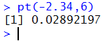
1. The first problem becomes P(X < -2.34) for 6 degrees of freedom.
The R statement to get this value, pt(-2.34,6),
and the answer are
shown in Figure 17.
Figure 17
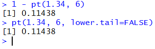
2. The second problem becomes P(X > 1.34)
for 6 degrees of freedom.
The R statement to get this value, 1 - pt(1.34, 6),
and the answer are
shown in Figure 18.
Alternatively, we could use the command pt(1.34, 6, lower.tail=FALSE)
to get the same result. That too is shown in Figure 18.
Figure 18
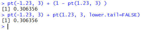
3. The third problem becomes
P(X < -1.23 or X > 1.23)
for 3 degrees of freedom.
The R statement to get this value,
pt(-1.23, 3) + (1 - pt(1.23, 3) ),
and the answer are
shown in Figure 19.
Alternatively, we could use the command
pt(-1.23, 3) + pt(1.23, 3, lower.tail=FALSE)
to get the same result. That too is shown in Figure 19.
Figure 19
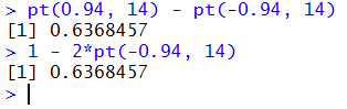
4. The fourth problem becomes
P( -0.94 < X < 0.94)
for 14 degrees of freedom.
The R statement to get this value,
pt(0.94, 14) - pt(-0.94, 14),
and the answer are
shown in Figure 20.
Alternatively, we could exploit the symmetry of the distribution and
use the command
1 - 2*pt(-1.23, 14)
to get the same result. That too is shown in Figure 18.
Figure 20
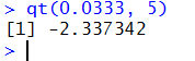
5. The fifth problem becomes find a value for t such that
P(X < t) = 0.0333 for 5 degrees of freedom.
The R statement to get this value, qt(0.0333, 5),
and the answer are
shown in Figure 21.
Figure 21
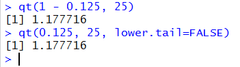
6. The sixth problem becomes find a value for t such that
P(X > t) = 0.125 for 25 degrees of freedom.
The R statement to get this value, qt(1 - 0.125, 25),
and the answer are
shown in Figure 22.
Alternatively, we could use the command
qt(0.125, 25, lower.tail=FALSE)
to get the same result. That too is shown in Figure 22.
Figure 22
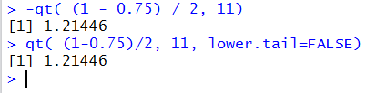
7. The seventh problem becomes find a value for positive t such that
P(-t < X < t)= 0.75 for 11 degrees of freedom.
The R statement to get this value, -qt( (1 - 0.75) / 2, 11),
and the answer are
shown in Figure 23.
Alternatively, we could exploit the symmetry of the
Student's t and use the command
qt( (1-0.75)/2, 11, lower.tail=FALSE)
to get the same result. That too is shown in Figure 23.
Figure 23
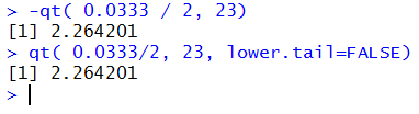
8. The eighth problem becomes find a value for positive t such that
P(X < -t) + P(X > t)= 0.0333 for
23 degrees of freedom.
The R statement to get this value,
-qt( 0.0333 / 2, 23),
and the answer are
shown in Figure 24.
Alternatively, we could use the command
qt( 0.0333/2, 23, lower.tail=FALSE)
to get the same result. That too is shown in Figure 24.
Figure 24
Review for pt and qt
Listing of all R commands used on this page
# Display the Student's t distributions with 2
# degrees of freedom and compare to the normal distribution
# Modeled after http://www.statmethods.net/advgraphs/probability.html

# a graph for 2 degrees of freedom

x <- seq(-4, 4, length=400)
hx <- dnorm(x)

degf <- 2
colors <-  c("red",  "black")
labels <- c("df=2",  "normal")

plot(x, hx, type="l", lty=2, lwd=2, xlab="z or t value",
     ylab="Density",
     main="Comparison of Normal and t Distribution \n 2 Degrees of Freedom"
     )

for (i in 1:1){
  lines(x, dt(x,degf[i]), lwd=2, col=colors[i])
}
abline(h=0)
abline(h=seq(0.1,0.4,0.1),lty=3, col="darkgray")
legend("topright", inset=.05, title="Distributions",
       labels, lwd=2, lty=c(1, 2), col=colors)


# a graph for 5 degrees of freedom

degf <- 5
colors <-  c("blue",  "black")
labels <- c("df=5",  "normal")

plot(x, hx, type="l", lty=2, lwd=2, xlab="z or t value",
     ylab="Density",
     main="Comparison of Normal and t Distribution \n 5 Degrees of Freedom"
)

for (i in 1:1){
  lines(x, dt(x,degf[i]), lwd=2, col=colors[i])
}
abline(h=0)
abline(h=seq(0.1,0.4,0.1),lty=3, col="darkgray")
legend("topright", inset=.05, title="Distributions",
       labels, lwd=2, lty=c(1, 2), col=colors)


# a graph for 8 degrees of freedom

degf <- 8
colors <-  c("darkgreen",  "black")
labels <- c("df=8",  "normal")

plot(x, hx, type="l", lty=2, lwd=2,xlab="z or t value",
     ylab="Density",
     main="Comparison of Normal and t Distribution \n 8 Degrees of Freedom"
)

for (i in 1:1){
  lines(x, dt(x,degf[i]), lwd=2, col=colors[i])
}
abline(h=0)
abline(h=seq(0.1,0.4,0.1),lty=3, col="darkgray")
legend("topright", inset=.05, title="Distributions",
       labels, lwd=2, lty=c(1, 2), col=colors)


# a graph for 15 degrees of freedom

degf <- 15
colors <-  c("darkorange",  "black")
labels <- c("df=15",  "normal")

plot(x, hx, type="l", lty=2, lwd=2,xlab="z or t value",
     ylab="Density",
     main="Comparison of Normal and t Distribution \n 15 Degrees of Freedom"
)

for (i in 1:1){
  lines(x, dt(x,degf[i]), lwd=2, col=colors[i])
}
abline(h=0)
abline(h=seq(0.1,0.4,0.1),lty=3, col="darkgray")
legend("topright", inset=.05, title="Distributions",
       labels, lwd=2, lty=c(1, 2), col=colors)


# a graph for 2, 5, 8, and  degrees of freedom


degf <- c(2,5,8,15)
colors <-  c("red", "blue", "darkgreen", "darkorange", "black")
labels <- c("df=2","df=5","df=8", "df=15",  "normal")

plot(x, hx, type="l", lty=2, lwd=2,xlab="z or t value",
     ylab="Density",
     main="Comparison of Normal and t Distribution \n 2, 5, 8, 15 Degrees of Freedom"
)

for (i in 1:4){
  lines(x, dt(x,degf[i]), lwd=2, col=colors[i])
}
abline(h=0)
abline(h=seq(0.1,0.4,0.1),lty=3, col="darkgray")
legend("topright", inset=.05, title="Distributions",
       labels, lwd=2, lty=c(1, 1, 1, 1, 2), col=colors)


## samples of pt() to compare
# with values shown on the web page
pt(-2.0,2)
pt(-2.0,15)
pt(-2.0,40)
pt(-2.0,100)

#
# examples using the upper tail
pt(3.078,1,lower.tail=FALSE)
pt(2.353,3,lower.tail=FALSE)
pt(4.604,4,lower.tail=FALSE)
pt(3.365,5,lower.tail=FALSE)

#
# samples of qt() to compare
# with values shown on the web page
qt(0.10,1)
qt(0.05,3)
qt(0.005,4)
qt(0.001,5)

#
# examples using the upper tail
qt(0.10, 1, lower.tail=FALSE)
qt(0.05, 3, lower.tail=FALSE)
qt(0.005, 4, lower.tail=FALSE)
qt(0.001, 5, lower.tail=FALSE)


#
# the eight worked examples
pt(-2.34,6)

1 - pt(1.34, 6)
pt(1.34, 6, lower.tail=FALSE)

pt(-1.23, 3) + (1 - pt(1.23, 3) )
pt(-1.23, 3) + pt(1.23, 3, lower.tail=FALSE)

pt(0.94, 14) - pt(-0.94, 14)
1 - 2*pt(-0.94, 14)

qt(0.0333, 5)


qt(1 - 0.125, 25)
qt(0.125, 25, lower.tail=FALSE)

-qt( (1 - 0.75) / 2, 11)
qt( (1-0.75)/2, 11, lower.tail=FALSE)


-qt( 0.0333 / 2, 23)
qt( 0.0333/2, 23, lower.tail=FALSE)
Return to Topics page
©Roger M. Palay
Saline, MI 48176 December, 2015