Probability: Normal approximation of the Binomial

Return to Topics page
Moving on from looking at probabilities related to proportions, we recognize that the binomial distribution must be related to that proportion distribution. After all, in a binomial distribution we report the number of successes out of some number of trials. In a proportion we report the quotient of the successes over the trials. As a result, we find that if we do repeated random samples of n trials then the mean of the count of success, denoted as μ_X, will approach n*p where p is the binomial probability of success on any one trial. Furthermore, the standard deviation of the count of successes, denoted as σ_X, will approach √n*p*(1-p).

We add to those facts the idea that under certain conditions, namely, when we have both n*p ≥ 10 and n*(1-p) ≥ 10, the binomial distribution can be approximated by a normal distribution with mean=μ_X = n*p and standard deviation=σ_X = √n*p*(1-p).

A small note is in order here. This "approximation" was almost essential before we had calculators and computers. Working out binomial probabilities using the binomial formula involved an enormous amount of multiplication. If you did not plan the evaluation of values correctly, those products could easily exceed 15 digits. You also had to raise the values p and (1-p) to high powers. Having a normal approximation to replace the evaluating those expressions was a real gift. However, we do have calculators and we do have computers, and the software has been tuned to do these problems directly and efficiently. This topic is presented here because we have been teaching it so long that we have forgotten why we do it. Sorry.

Let us walk through an example. We start with a coin that has a probability of 0.68 that it will come up "tails" on a fair spin. If we spin the coin 150 times, what is the probability that we will have less than 93 tails? With such a high number of spins we will use the normal approximation to the binomial distribution. First, we need to check that n*p ≥ 10 and n*(1-p) ≥ 10. We have n = 150 and p = 0.68 giving n*p = 150*0.68 = 102 ≥10 and n*(1-p) = 150*0.32 = 48 ≥ 10. We can move forward. The mean = n*p = 102 and the standard deviation = √n*p*(1-p) = √150*0.68*0.32 ≈ 5.713143. The R statement to find the desired value is pnorm(92.5,mean=102,sd=5.713143). A similar statement, along with supporting computations, is found in Figure 1.

Figure 1

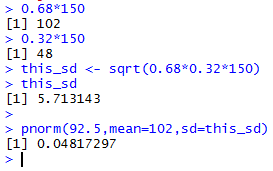
Note that we used 92.5 because the normal distribution is continuous while the binomial distribution is discrete.

By the way, since we do have R and we know that R has the pbinom function, we could have computed the straight binomial probability by using the command pbinom(92,150,0.68) as is shown in Figure 1a.

Figure 1a

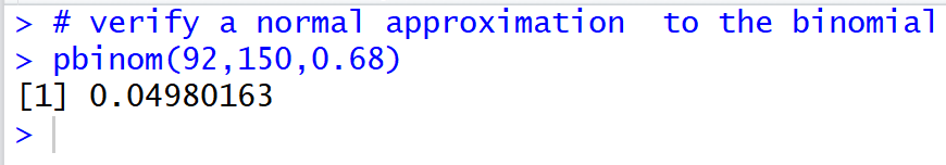
Note how close our normal approximation to the binomial in Figure 1 is to the computed value shown in Figure 1a.

Using the same coin, we could move to answering such questions as

For the 150 spins, what is the probability that we will get more than 108 tails?
For the 150 spins, what is the probability that we will get between 105 and 109 tails, inclusive?
For the 150 spins, what is the probability that we will get fewer than 98 tails or more than 107 tails?

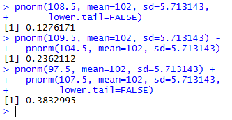
The R commands to get those values would be

pnorm(108.5, mean=102, sd=5.713143, lower.tail=FALSE)
pnorm(109.5, mean=102, sd=5.713143) - pnorm(104.5, mean=102, sd=5.713143)
pnorm(97.5, mean=102, sd=5.713143) + pnorm(107.5, mean=102, sd=5.713143, lower.tail=FALSE)

Those commands are shown in Figure 2.

Figure 2

As we have done in the past, it would be easier to create a function that does all of the preliminary work for us, saving us from having to remember to do those checks as well as computing the mean and standard deviation that we need for the pnorm() function. Such a function is:

pnormbino <- function( num_success, p, n, lower.tail=TRUE)
{
  if(p*n < 10) {return("n*p < 10, will not compute this")}
  if(n*(1-p) < 10)
  {return("n*(1-p)<10, will not compute this")}
  nbsd <- sqrt( n*p*(1-p))
  prob <- pnorm(num_success, n*p, nbsd, lower.tail)
  return( prob )
}

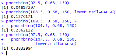
Figure 3 shows the same problems as before, but solved with calls to the new pnormbino() function.

Figure 3