Probability: Proportions
Return to Topics page
The proportion of items in a population that have some specified
characteristic is the quotient of the number of items in the population with
that characteristic
divided by the population size.
We use  to represent the population proportion.
The proportion of items in a sample that have some specified
characteristic is the quotient of the number of items in the sample with
that characteristic, x,
divided by the sample size.
We use  , read as "p hat",
to represent the sample proportion. In symbols we have
, read as "p hat",
to represent the sample proportion. In symbols we have

As we might expect, if we took repeated samples of size n
then the mean of the sample proportions would approach the
population proportion.
That is,

It would also be the case that the standard deviation of the
sample proportions would approach the following value:
There is an interplay between the size of p and the size of n
such that in special cases, hopefully in any case we use,
if n*p ≥ 10 and n*(1-p) ≥ 10 then
the distribution of
is approximately normal with
mean= and
standard deviation=
and
standard deviation= .
That approximation means that, in those cases, we can use the normal
table and/or the R functions pnorm() and qnorm()
to answer questions about the probability of certain random events involving
proportions in random samples of a population.
.
That approximation means that, in those cases, we can use the normal
table and/or the R functions pnorm() and qnorm()
to answer questions about the probability of certain random events involving
proportions in random samples of a population.
For example, if we know that 74% of the students in introductory
engineering courses are males, then, in a random sample of 94 students
in such classes what is the probability that the sample will have
80% or more males? The 74% in the population makes
p=0.74. That makes (1-p)=0.26.
With n=94 we confirm that np≥10
and n(1-p)≥10, with values of 69.56 and 24.44,
respectively.
Therefore, we can use a normal approximation with
μ=p=0.74 and
σ=sqrt(p(1-p)/n)=sqrt(0.74*0.26/94)≈0.04524.
In order to use the standard normal table
we need to change the 80% to a z-score,
 ,
to get z=(0.80-0.74)/0.04524≈1.326.
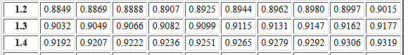
Then, look at the standard normal table, a portion of which
is shown in Figure 1. We cannot find our z value, 1.326,
exactly in the table because the table is only good for 3 places.
The best the table can do is to get us close to 1.326.
That is, we can find values for 1.32 and 1.33.
From the table we see that the area to the left of 1.32
is about 0.9066 while the area to the left of 1.33 is about 0.9082.
,
to get z=(0.80-0.74)/0.04524≈1.326.
Then, look at the standard normal table, a portion of which
is shown in Figure 1. We cannot find our z value, 1.326,
exactly in the table because the table is only good for 3 places.
The best the table can do is to get us close to 1.326.
That is, we can find values for 1.32 and 1.33.
From the table we see that the area to the left of 1.32
is about 0.9066 while the area to the left of 1.33 is about 0.9082.
Figure 1
For 1.326 we want to move 6 tenths of the way
from the former toward the latter.
0.9082 - 0.9066 = 0.0016, and 0.6*0.0016=0.00096
so our answer for the area to the left of
80% would be 0.9066+0.00096=0.90756.
Of course, we want the area to the right of that value and that
would be 1 - 0.90756 = 0.09244.
Therefore, the probability of having 80% or more males is about 9.244%,
remembering that we had to use various rounded values.
Then again, because we have been paying attention and because we have
R, we could just form the command
pnorm(0.80, mean=0.74, sd=sqrt(0.74*0.26/94), lower.tail=FALSE),
as shown in Figure 2, and get the same, though a bit more accurate, result.
In either case we are not going to report all the extra digits. We would round both answers
to say that the probability is 9.24%.
Figure 2

Clearly, using the pnorm() function in R is much easier than
going through all of that work getting the z-score,
looking up values, interpolating, and then, in this case, getting the
complementary value. Still, we would have to remember just how to
form that pnorm() command. Then again, the form does not change, just the
values that we are using. Those values are the
sample proportion, the population proportion, the sample size,
and do we want to use the left or the right tail?
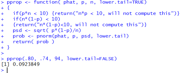
Why not just create our own function for this.
We could do something like
pprop <- function( phat, p, n, lower.tail=TRUE)
{
  if(p*n < 10) {return("n*p < 10, will not compute this")}
  if(n*(1-p) < 10)
  {return("n*(1-p)<10, will not compute this")}
  psd <- sqrt( p*(1-p)/n)
  prob <- pnorm(phat, p, psd, lower.tail)
  return( prob )
}
And then the problem becomes one of just giving the command
pprop(.80, .74, 94, lower.tail=FALSE).
All of this is shown in Figure 3.
Figure 3
You might note that the function definition uses
lower.tail=TRUE. This was done to keep pprop()
similar to pnorm() and pt().
Also, our function saves us from trying to apply the
approximation in cases where it does not fit.
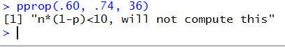
Were we to have a case where 74% of the students were male and
we had a sample of size 36, then the value of 36*(1-0.74) would
not be greater than or equal to 10. That tells us that we cannot
apply the normal approximation, no matter what sample proportion
we want to evaluate.
To find the probability that the sample
has 60% of fewer males we would give the command
pprop(.60, .74, 36) which would just return the message
"n*(1-p)<10, will not compute this" as shown in Figure 4.
Figure 4
Some note should be made here about problem statements that do not give you
the probabilities for having the characteristic or not having it, that is, they do not
give you p and therefore (1-p). For example,
we might be told that from a population of 1256 individuals we have a sample
that contains 13 males and 21 females. Could we use or normal approximation for
proportions in this case? First, we note that our sample size is 34 (the total of males and
females). 34 is less than 5% of our population (0.05*1256 is 62.8). We need to
be sampling less than 5% in order to ignore the changes in probabilities when we
sample without replacement. Second, if we knew the proportion of males,
call it pm, and the proportion of
females, call it pf, so
pm+pf=1,
then we would need n*pm≥10 and
n*pf≥10 in order to use the normal approximation.
Since we do not know pm or
pf we will use 15/34 for
pm and 21/34 for
pf. Then our requirement that
n*pm≥10 becomes 34*(15/34)≥10 and our
requirement that
n*pf≥10 becomes 34*(21/34)≥10.
Note that in both cases the 34's cancel and what is left is that the
number of males must be greater than or equal to 10 and the number
of females must be greater than or equal to 10. In short, looking at the original problem statement
we did not have to go through all that computation, we just needed to be sure that we
had at least 10 items with the characteristic and at least 10 items without the characteristic.
Here are three more examples, but we will use pprop() to solve them.
Figure 5 gives data taken from the Center for Disease Control web page.
Figure 5

According to Figure 5 about 20% of people ages 18 to 24 years
in Michigan reported smoking every day or some days in 2013.
In a random sample of size 36 of
people who lived in Michigan in 2013 and who were 18 to 24 then,
what is the probability that 5 or fewer of them smoked every day of some days?
We will just fill in the pprop() statement to do this.
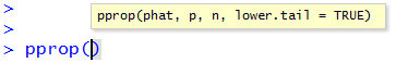
We start by typing, in our R session, pprop(.
R immediately fills in the closing parenthesis and shows a helpful
guide giving the function parameters. This is shown in Figure 6
Figure 6
We see that the first parameter is phat. To supply this we need to
type 5/36. The second and third parameters are p and n,
for which we supply .20 and 36. The fourth parameter shows that its
default value is TRUE. This is the value that we want so we do not even need to supply it.
Thus our complete command becomes the pprop(5/36, 0.20, 36)
shown, with the result, in Figure 7.
Figure 7
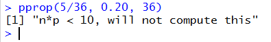
The system has saved us from making a mistake!
If we change the problem, slightly, and ask in a sample of size 72
of these same people what is the probability of getting 10 or fewer
smokers, then the command becomes the
pprop(10/72, 0.20, 72)
shown, with the result, in Figure 8.
Figure 8
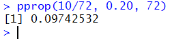
It is interesting to note that we doubled the sample size and
left the proportion the same (5/36=10/72) but now we have enough
in the sample to use the approximation.
Figure 9 presents data taken from another CDC page.
Figure 9

If 31% of all traffic-related deaths in 2013 were in alcohol-impaired
driving crashes and we take a sample of 58 driving crashes from 2013,
what is the probability that between 15 and 45 of those crashes
will have been deemed alcohol-impaired? We will do this by saying that the
answer will be P(X ≤ 45) - P(X < 15).
Wait a minute! Why use ≤ in one place and < in the other?
This immediately opens our eyes to an issue that we ignored in
doing the previous problem. In particular, since the normal
distribution is continuous, we recall that the P(X = 15)=0.
Our first analysis seems flawed. We should restate the problem as
P(X < 45.5) - P(X < 14.5).
We should have done a similar change in the previous problem, but
we are just too lazy to go back and fix that. Well maybe we can sneak an update
into the answer to this one, shown in Figure 10.
Figure 10
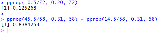
Figure 10 gives an improved interpretation to the earlier problem (resulting in changing
that answer to 12.5%), and an answer to this problem, namely, 83.84%.
The information in Figure 11 was taken
from the Bureau of Transportation Statistics.
Figure 11
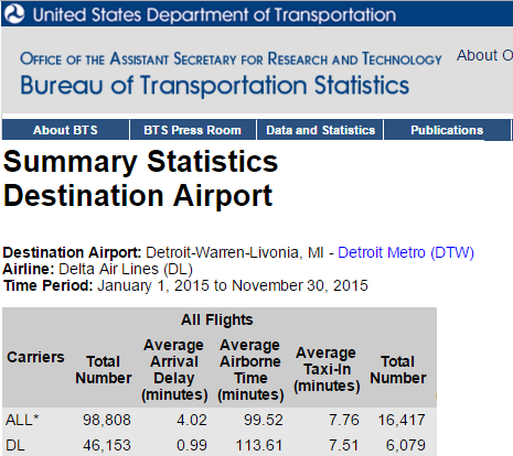
With that information in mind, for a sample of 85 random Delta flights
between 01/01/2015 and 11/30/2015 with a destination of Detroit (DTW),
what is the probability that there will be less than 5 or more than 80
delayed flights in the sample?
We use the pprop() to do this as the sum of the
probability of the two cases, taking into account
the offset between whole number values.
This is shown in Figure 12.
Figure 12
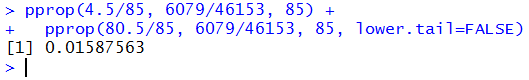
Those are pretty extreme values, so we are not shocked to see such a small
probability, 1.588%, as the answer.
Return to Topics page
©Roger M. Palay
Saline, MI 48176 December, 2015