Probability: Continuous Cases

Return to Topics page
There is a reason that we do not use continuous cases when we first start talking about probability distributions. Discrete cases are nice because we can assign a definite probability to each case. We cannot do this for continuous cases. Part of the reason for this is that there are no "cases" with a continuous sample space. For example, the height of people is a continuous measure. When we give our height we approximate it by rounding it off to a discrete value. I might say I am 5 foot 11.5 inches tall. Now the truth is, I am not 5 foot 11.5 inches tall. I am close to that. I am very close to that. But I am absolutely sure that if I got a really good measurement of my height, I would not be exactly 5 feet 11.5 inches tall.

The same is true for the age of people. When someone says that they are 23 years old, it is almost certain that they are not telling the complete truth. In order to be exactly 23 years old, today must be the birthday of that person! If her/his birthday was a week ago then she/he is 23 years and 1 week old. Well, that is also most likely not true. If she/he were born 23 years and 1 week ago, but two hours earlier than now, then she/he is 23 years, 1 week, and 2 hours old. Well strictly speaking, that is also most likely not true because we could look to the minute, to the second, to the tenth of a second, and so on.

The point is that for continuous measures it is essentially impossible to find any single exact value. To put this more bluntly, this term at WCC there are probably over 1000 students who would say that they are 19. It is almost certain that not even one of them is actually 19 as of the moment that you read this.

In the discrete cases we could assign a probability to each case. In continuous cases, since there are no real exact values, we need to find another way to talk about probabilities. Whereas it would be almost impossible for the next WCC student that you meet to be exactly 23 years old, there is no problem saying that the next WCC student who you meet is less than 23 years old. This is the strategy that we will use for continuous values.

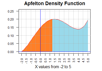
Consider the graph in Figure 1. The curve on this figure has a point for every value between -2 and 5. These are the only values that are defined for the domain of the Apfelton distribution.

Figure 1

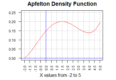
The height of the curve above any point is interesting, but it is not the central feature of the graph. What is important is to note that the area under the curve (to the right of -2, to the left of 5, above the x-axis, and below the red curve) is equal to 1 unit. Each rectangle outlined in Figure 1 is 0.5 units wide and 0.05 units tall (the scales for horizontal and vertical are not the same). Therefore, each rectangle is 0.025 square units.

We can approximate the area under the curve by counting the rectangles below it. Figure 2 shows such an approximation. Many of the rectangles in Figure 2 are clearly under the curve, for example, rectangles 2, 4, 5, 11, and 38. Rectangle #3 is mostly under the curve, but the green portion of that rectangle is above the curve. Also, there are some rectangles without a number that still have part of the rectangle below the curve. For example, the rectangle to the left of rectangle #1 has its blue area under the curve, but most of that rectangle is above the curve. Thus, the green areas are part of the 39 rectangles but not under the curve and the blue areas are under the curve but not part of any numbered rectangle.

Figure 2

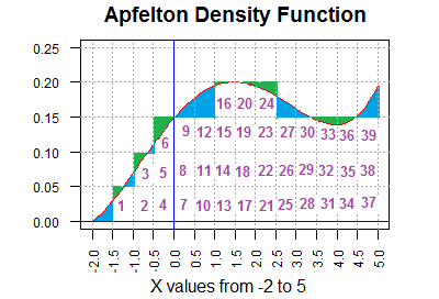
Thus, the total area under the curve is the area of the 39 numbered rectangles minus the area that is shaded green plus the area that is shaded blue. It turns out that the total blue area is bigger than is the total green area. In fact, it is bigger by exactly 1 rectangular region. Therefore, the area under the curve is 40*0.025 = 1.00 square unit.

We do know that the total probability for the entire sample space of any problem must be 1.00. Therefore, the area under the curve is a good representation of probability for the Apfelton distribution. We can use that concept to say that the probability of randomly selecting an item (a value) from the Apfelton distribution and having that item be less than 1.5 is equal to the area under the curve and less than the vertical line at 1.5. A picture of this is given in Figure 3.

Figure 3

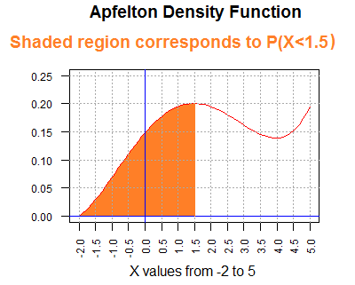
We could approximate this area by counting rectangular areas again, but such is not a particularly speedy nor accurate way to get a value for that area. We do know, however, that the area is greater than 0 and less than 1. In fact, using the counting that we did in Figure 2, the shaded area in Figure 3 should be a little more than 16 rectangular areas (each 0.025 square units). But 16*0.025 is 0.4, so we have a rough approximation of 0.4 as the probability of getting a value less than 1.5 in an Apfelton distribution. The true answer, by the way, is 0.4165.

How do you get the true answer? In the "old days" we would use a table of values. The skill to use a table, while a bit archaic in these days of calculator and computer software, is still very much a part of this course. I have a web page that provides such a table. The following link should open a new tab so that you can switch back and forth quickly between there and here. That link is "The Apfelton Distribution."

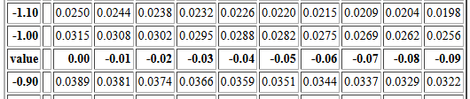
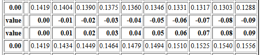
The table is arranged with increasing "values" in the left column. Those values increase by 0.1 for each row. The first number to the right of those values is the P(X<value). Continuing to the right we find nine more values, each one corresponding to PX<value+offset) where offset takes on successive values -0.01, -0.02, -0.03 and so on, at least for the top portion of the table. For example, P(X<-1.00)=0.0315. Reading to the right, P(X<-1.01)=0.0308, P(X<-1.02)=0.0302, P(X<-1.03)=0.0295, and so on. That portion of the table is reproduced in Figure 4.

Figure 4

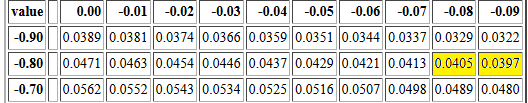
Please notice that there are two rows that have the value 0.00 in the left column. Of those two rows the top row gives probabilities associated with the values 0.00, -0.01, -0.02, -0.03, ... -0.09. After that the offset is restated and then the offset is changed to 0.00, 0.01, 0.02, 0.03, ... 0.09. Then the second row starting with 0.00 gives the probabilities associated with the values 0.00, 0.01, 0.02, 0.03, ... 0.09. Those rows are reproduced n Figure 5.

Figure 5

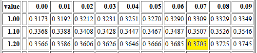
To find P(X<1.27) we find the row that starts with the value 1.2. Then we read across until we are in the 0.07 offset column. That value is 0.3705. Therefore, P(X<1.27)=0.3705. That area of the table is reproduced in Figure 6 with the particular cell of the table highlighted.

Figure 6

One might ask for the P(X = 1.27). The table will not help us on that. The table only gives the area under the probability density curve and to the left of a given value. The table tells is that P(X<1.27)=0.3705 but gives us little help in finding P(X = 1.27).

Well, the table does give us the answer, but it might not be the one you expect. The table represents probability as area. There is no rectangular region above the single value 1.07; Figure 1 shows that there is a line segment that reaches up to a value close to 0.20, but a line segment has no width. Area is length times width. If the width is 0 then the area is 0. We correctly say that P(X = 1.27)=0. You should note that this corresponds to the concept expressed near the top of this page: it is essentially impossible to find any exact value in a continuous distribution.

As a result of this, for any value v it is always true that P(X ≤ v) = P(X < v).

Although the Apfelton table only gives probabilities for random values less than a specific value, we can use the same table to find probabilities such as P(X > 1.27) or P(-1.03 < X <1.27) or P(X < -1.03 or X > 1.27).

To find P(X > 1.27) we recall that the entire area under the curve is 1 square unit. We want the area shaded light blue in Figure 7. The table gives us the area shaded in orange in that figure. Thus, the area shaded in light blue is equal to 1 minus the area shaded in orange.

Figure 7

Mathematically stated, P(X > 1.27) = 1 - P(X < 1.27) but the table gives us P(X < 1.27) = 0.3705 so P(X > 1.27) = 1 - 0.3705 = 0.6295.

To find P(-1.03 < X <1.27) means finding the area of the orange region in Figure 8.

Figure 8

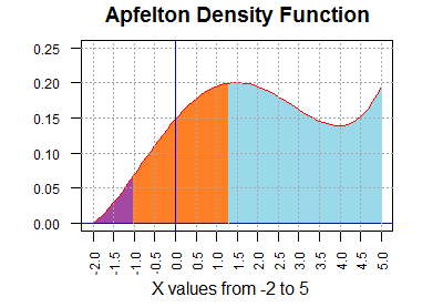
We look up P(X < 1.27) in the table. That gives us the area of the combined orange and purple region. If we look up P(X < -1.03) in the table that gives us the area of just the purple region. Therefore, the area of the orange region is the area of the combined orange and purple region minus the area of the purple region.

Mathematically stated, P(-1.03 < X <1.27) = P(X <1.27) - P(X < -1.03) but the table gives us P(X < 1.27) = 0.3705
P(X < -1.03) = 0.0295 so P(-1.03 < X <1.27) = 0.3705 - 0.0295 = 0.3410

To find P(X < -1.03 or X > 1.27). means finding the area of the combined light blue and purple regions in Figure 8. We could do this as finding the area of the purple region, P(X < -1.03) and add to that the area of the light blue region which we found to be 1 - P(X < 1.27), which we would express as P(X < -1.03 or X > 1.27) = P(X < -1.03) + (1 - P(X < 1.27) )
P(X < -1.03 or X > 1.27) = 0.0295 + (1 - 0.3705)
P(X < -1.03 or X > 1.27) = 0.0295+0.695
P(X < -1.03 or X > 1.27) = 0.6590 or we could just say that the area of the combined light blue and purple regions is 1 minus the area of the orange region which we would express as P(X < -1.03 or X > 1.27) = 1 - (P(X < 1.27) - P(X < -1.03) )
P(X < -1.03 or X > 1.27) = 1 - (0.3705 - 0.0295)
P(X < -1.03 or X > 1.27) = 1 - (0.3410)
P(X < -1.03 or X > 1.27) = 0.6590
All the examples above used the table to find the probability that our random variable from the Apfelton distribution is less than some value. We could, however, use the table backwards, starting from a given probabiity and answering the question "What value from the distribution has that area to its left?"

For example, if we have P(X < v) = 0.04 then we can use the table, backwards, to find the value of v. To do this we find the value 0.04 or at least the values that surround it, in the table. Figure 9 shows the part of the table that contains the two table cells that surround 0.04, namely, 0.0405 and 0.0397, both of which are highlighted in Figure 9.

Figure 9

Then we identify the values that are linked to those to cells. In particular, -0.88, which has P(X <-0.88) = 0.0405, and -0.89, which has P(X <-0.89) = 0.0397. Clearly, the value that we want, the value that satisfies P(X < v) = 0.04 must be between -0.88 and -0.89. The difference between the cell values 0.0405 and 0.0397 is 0.0008. Moving from 0.045 to 0.0397 we only want to move 0.0005. If we are to believe the values in the table cells then we could interpolate a value that is 0.0005/0.0008 = 5/8 of the way between -0.88 and -0.89. Since 5/8 = 0.625 our interpolated answer would be -0.88625, an answer with far more accuracy than it deserves. Really, we should add at most 1 digit not the 3 that we used. Therefore, our answer will be -0.886.

Why would we say "If we are to believe the values in the table cells..."? We say that because the although the table is correct, the values in the table are rounded to 4 decimal places. We are using those rounded values in our interpolation. As we will see below more accurate values are

P(X < -0.88) ≅ 0.04049132
P(X < -0.89) ≅ 0.03969926
P(X < -0.886) ≅ 0.04001508
P(X < -0.8861905886) ≅ 0.04000000005353

However, if the table is all that we have then we just use the table values knowing that we are quite close to the correct answer.

The examples above should make it clear that we can use the Apfelton Distribution Table to answer many different probability questions about that continuous distribution. Of course, having the table does not tell us how the values in the table were computed. As it turns out, the Apfelton distribution is determined by a mathematical formula: f(v) = (v⁴-4*v³-15*v²+58*v+128)/862.4 This, however, means that we have a probability function, p(v) defined as p(v) = ((1/5)v⁵-v⁴-5*v³+29*v²+128*v+122.4)/862.4 where p(v) gives us the value in the table for v, that is p(v) = P(X < v).

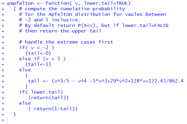
That is a nice mathematical function, and we can implement that function in R. The code for such a function, one that is slightly enhanced, is

papfelton <- function( v, lower.tail=TRUE)
  { # compute the cumulative probability 
    # for the Apfelton distribution for vaules between
    # -2 and 5 inclusive.
    # By default return P(X < v), but if lower.tail=FALSE
    # then return the upper tail
  
    # handle the extreme cases first
    if( v < -2 )
      {tail<-0}
    else if (v > 5 )
      {tail<-1}
    else
      {
       tail <- (v^5/5 - v^4 -5*v^3+29*v^2+128*v+122.4)/862.4
      }
    if( lower.tail)
       {return(tail)}
    else
       { return(1-tail)}
  }

The name, starting with the letter p, and the slight enhancement, adding an optional parameter lower.tail, follow the style of similar functions that are available in R for the standard distributions.

Figure 10 shows the console image of the same function as it was added to a RStudio session.

Figure 10

Once the function papfelton() is defined we can use it to calculate all of the various probabilities that we looked up in the table. Figure 11 shows the single values values that we had found above. it is worth comparing these values to the ones taken from the table.

Figure 11

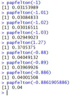
The computed values have many more significant digits. Now we can see that the table values are indeed rounded to 4 decimal places. For example, our table value for P(X < 1.27) ) was 0.3705 but the function returns the more accurate value of 0.3705375.

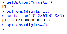
It is interesting to note that Figure 11 shows R computing papfelton(-0.8861905886) to be 0.04 but we had noted above, that the more accurate value is 0.04000000005353. The difference is determined by the number of significant digits that R is trying to display. By default, that number is 7. In fact, all the other results in Figure 11 have 7 significant digits. However, when R rounds off 0.04000000005353 to 7 significant digits the result is a number with all trailing 0's, and R chooses to display that simply as 0.04.

Figure 12 demonstrates the effect of changing the setting in R for suggested number of digits to display as well as showing the full 13 significant digits of 0.04000000005353.

Figure 12

There are a number of inconsistent styles between the commands getOption("digits") and options(digits=13). It is important to notice that

There is a capital O in getOption
There is no s in getOption
The argument in getOption is given as a string
The command options ends with the letter s
The argument in option is a simple "named" parameter such as digits

Starting just above Figure 7, the table related discussion above walked us through computing the more complex probabilities P(X > 1.27) or P(-1.03 < X <1.27) or P(X < -1.03 or X > 1.27). Now that we have the papfelton() function we can create expressions to do these too.

We had seen that P(X > 1.27) = 1 - P(X < 1.27) and we can do exactly that with the command 1-papfelton(1.27). That is the first command in Figure 13.

Figure 13

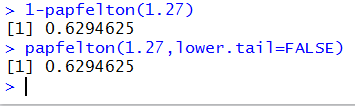
The second command in Figure 13 demonstrates the optional argument for papfelton(). We change the behavior of papfelton() from calculating the lower tail probability to calculating the upper tail probability by including the argument lower.tail=FALSE argument. In effect, papfelton(1.27,lower.tail=FALSE) computes P(X > 1.27). Of course, we get the same answer using either strategy.

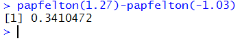
To find P(-1.03 < X <1.27), we use the fact that P(-1.03 < X <1.27) = P(X <1.27) - P(X < -1.03) and form the command papfelton(1.27)-papfelton(-1.03) as shown in Figure 14.

Figure 14

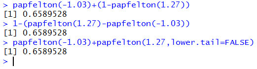
To find P(X < -1.03 or X > 1.27), we could use the fact that P(X < -1.03 or X > 1.27) = P(X < -1.03) + (1 - P(X < 1.27) ) or that P(X < -1.03 or X > 1.27) = 1 - (P(X < 1.27) - P(X < -1.03) )
and write these as papfelton(-1.03)+(1-papfelton(1.27)) or as 1-(papfelton(1.27)-papfelton(-1.03)). Alternatively, we could use the lower.tail=FALSE argument to just write this as papfelton(-1.03)+papfelton(1.27,lower.tail=FALSE). All three forms are shown in Figure 15.

Figure 15

So far we have seen that we can use the papfelton() command to do all of the the work that we learned to do in looking up values in the table. However, the last table skill that we learned was to use the table backwards. That is, if we are given a probability, say q, then we learned to find a value v such that P(X < v) = q. We need a way to do this without looking up the value in the table, and, along the way, to get a more accurate value for v.

The code for an inverse function, one we will call qapfelton(), is a bit more involved than codes that we have seen before. For our purposes it is not necessary for you to completely understand the inner workings of that code, but it is provided here both so that you can examine it if you want to do so and so that you have a source for it if you want to copy it and place it into an RStudio session. The code for qapfelton() is

qapfelton <- function( q, lower.tail=TRUE)
  { # inverse function of papfelton()
  if( q < 0 )
     { q <- 0 }
  else if ( q > 1 )
     {q <- 1 }
  if( !lower.tail )
     { q <- 1-q}
  # handle extreme cases
  if ( q == 0 ) {return(-2)}
  if ( q == 1 ) { return(5)}
  low <- -2
  high <- 5
  error <- 1
  while (error > 0.0000000001)
    { 
     next_v <- (low+high)/2
     next_p <- papfelton( next_v )
     if ( next_p <= q )
       { 
        low <- next_v
        error <- q - next_p
       }
     if ( next_p >= q )
     { 
       high <- next_v
       error <-  next_p - q
     }     
    }
  return( next_v )
  }

Again, the naming of the function and the inclusion of the optional parameter lower.tail=TRUE follow similar standard function within R for the standard distributions.

Once installed in our RStudio session, we can use the qapfelton() function by giving commands such as qapfelton(0.04) and qapfelton(0.5) as shown in Figure 16.

Figure 16

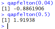
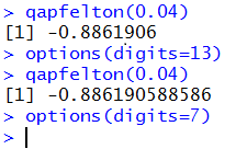
Now that you have seen two examples of the use of qapfelton() you can understand how we came to identify the value -0.8861905886 that we used as the best value to place into papfelton() in order to get a result really close to 0.04. All it took was to give the command qapfelton(0.04) as shown in Figure 17.

Figure 17

This page, to this point, used the Apfelton distribution. Here we introduce a new distribution, the Blumenkopf distribution not only as a vehicle to review what we saw above, but also to introduce a new twist in our discussion of probabilities and tables. The Blumenkopf Density graph is shown in Figure 18

Figure 18

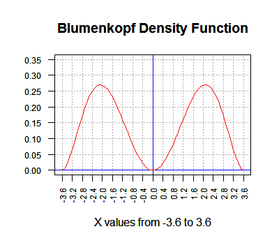
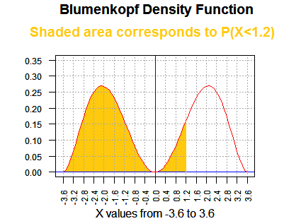
The interpretation of that graph is the same as it was for the Apfelton distribution earlier, except that the Blumenkopf distribution is defined for values from -3.6 to 3.6. Thus, the area under the curve is equal to 1 square unit. If we choose a value, say 1.2, then the area under the curve and to the left of our value, 1.2, is the probability of having the random variable from the Blumenkopf distribution be less than 1.2. That area is shown in Figure 18.

Figure 19

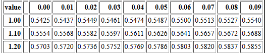
Then we want to see a table of the values of P(X < v) for values of v from -3.6 to 3.6. That table is at "The Blumenkopf Distribution".

From that table we note that P(X < 1.2) = 0.5703. The portion of the table that shows this is given in Figure 20.

Figure 20

Of course P(X < 1.2) = 0.5703 means that P(X > 1.2) = 1 - 0.5703 = 0.4297.

Now, let us look at P(X < -1.2). The portion of the table needed for that is given in Figure 21.

Figure 21

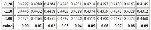
We see that P(X < -1.2) = 0.4297, the same value that we had for P(X > -1.2). This is not a coincidence! Pick any valid value v and you will find, for the Blumenkopf distribution, that 1 - P(X < v) = P(X < -v) This is true because the Blumenkopf distribution is symmetric about 0. If we were to print Figure 1 and then fold the paper along the y-axis (at x=0) the graph to the left of 0 would fit perfectly on top of the graph to the right of 0.

Of course, this means that half of the area is to the left of 0 and half is to the right. We can see that if we look at the portion of the table shown in Figure 22.

Figure 22

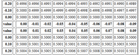
Looking at Figure 1 we see that there is almost no area under the curve close to 0. That is why the rounded to 4 places values in the table for values close to 0.0 are all displayed as 0.5000.

One small, though at times confusing, implication of this symmetry is that if we are going to create a table of values then we only need to create the table for values from 0.00 to 3.59. After all, we know that the table entry for 3.6 would be 1.0000, and the value for any negative value from -3.59 to 0.00 can be determined from the equation above as being 1 - P(X < posv) where posv is the positive reflection of the negative value. Only having to print half of a table would be an advantage if we were printing a book but it is essentially meaningless in terms of having a table on the web.

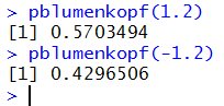
The Blumenkopf distribution is presented here because it is symmetric. We see how that symmetry can be used to shorten a table and how the relationship between positive and negative values can be expressed in an equation. Just to complete the treatment of the Blumenkopf distribution we will look at the pblumenkopf() and qblumenkopf() functions. The pblumenkopf() function gives the area under the curve to the left of the specified value. Thus, pblumenkopf(1.2) should produce 0.5703 as a confirmation of the value we found in the table, and pblumenkopf(-1.2) should produce 0.4297 both to confirm the table and to confirm our equation. The code for pblumenkopf() is given as

pblumenkopf <- function( v, lower.tail=TRUE)
{ # compute the cumulative probability 
  # for the Blumenkopf distribution for vaules between 
  # -3.6 and 3.6 inclusive.
  # By default return P(X < v), but if lower.tail=FALSE
  # then return the upper tail
  
  # handle the extreme cases first
  if( v < -3.6 )
  {tail<-0}
  else if (v > 3.6 )
  {tail<-1}
  else
  { E<-121741/159168+16
    tail <- (v^7/7-26*v^5/5+169*v^3/3)/(E*72)+0.5
  }
  if( lower.tail)
  {return(tail)}
  else
  { return(1-tail)}
}

Figure 23 shows the use of the function to confirm our earlier values from the table. Again, note the increased number of significant digits.

Figure 23

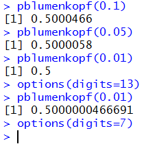
Now, with the extra digit we can return to the region around 0.00 to see if all those values in the table cells are really 0.5000. Figure 24 displays the more accurate values, although to see that the probability associates with 0.01 is not really 0.5 we had to increase the number of display digits.

Figure 24

If we are to use the Blumenkopf distribution then we want a function, qblumenkopf() that "reads the table backwards", that is, if we give it a probability, q, then it produces a value, v, such that P(X < v) = q. The code for qblumenkopf() is

qblumenkopf <- function( q, lower.tail=TRUE)
{ # inverse function of pblumenkopf()
  if( q < 0 )
  { q <- 0 }
  else if ( q > 1 )
  {q <- 1 }
  if( !lower.tail )
  { q <- 1-q}
  # handle extreme cases
  if ( q == 0 ) {return(-3.6)}
  if ( q == 1 ) { return(3.6)}
  low <- -3.6
  high <- 3.6
  error <- 1
  while (error > 0.00001)
  { 
    next_v <- (low+high)/2
    next_p <- pblumenkopf( next_v )
    if ( next_p <= q )
    { 
      low <- next_v
      error <- q - next_p
    }
    if ( next_p >= q )
    { 
      high <- next_v
      error <-  next_p - q
    }     
  }
  return( next_v )
}

Then, Figure 25 shows some examples of using qblumenkopf().

Figure 25

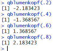
Again, the fact that qblumenkopf(.2) and qblumenkopf(.8) produce opposite values, as do qblumenkopf(.4) and qblumenkopf(.6), is because the Blumenkopf distribution is symmetric with respect to the 0 value.