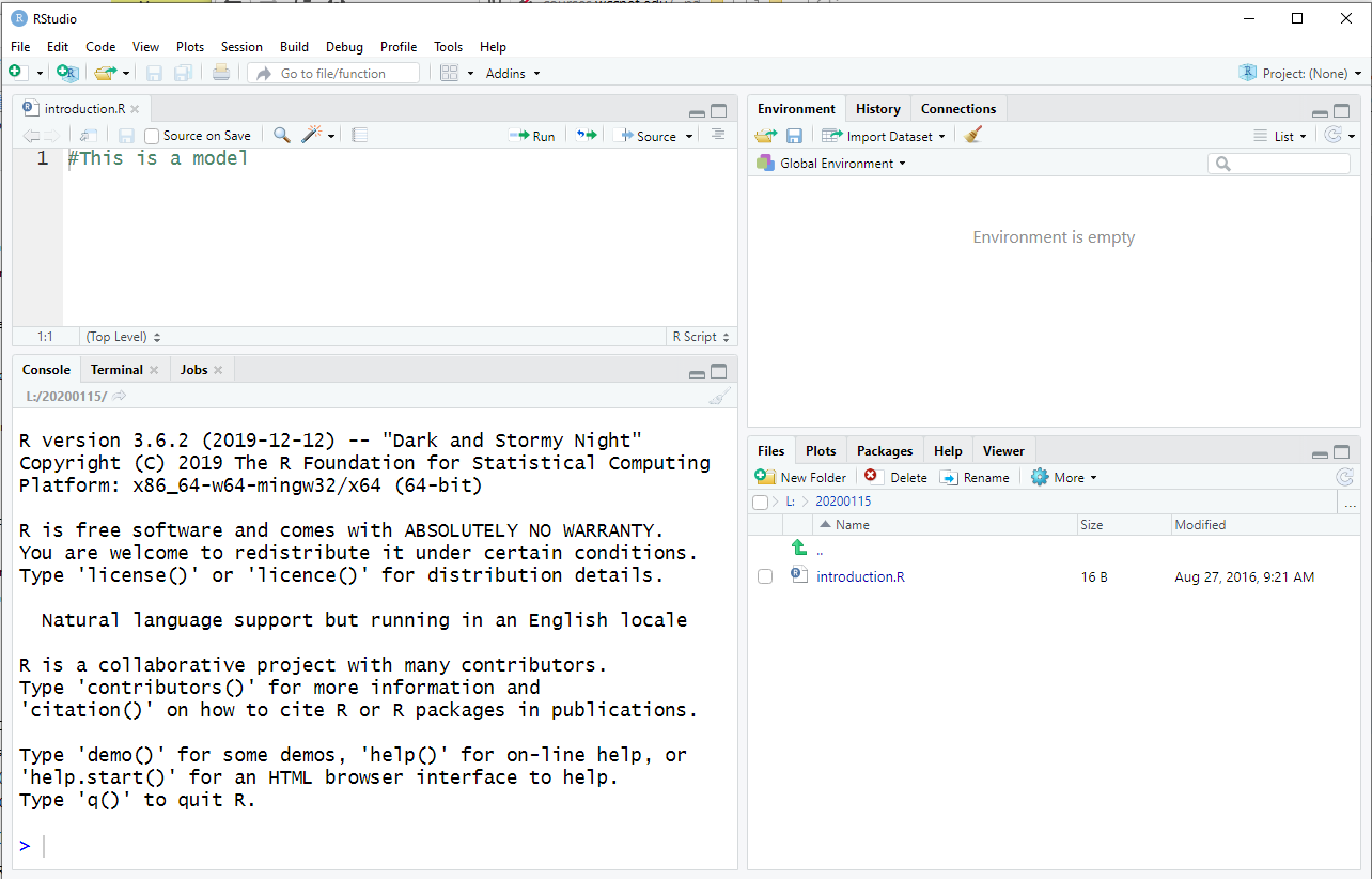
In order to use R there are a few things that we should experience, even before we start looking at the statistical side of the language. For this introduction I have used the Integrated Development Environment called RStudio. This IDE allows us to give R commands in one window pane and to see the effect of some of the commands in another pane. Figure 0 below shows the opening screen that we get when we start RStudio.
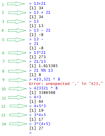
One of the things that we want to be able to do in R is to perform simple, or even not so simple, arithmetic operations. We can just enter the expression that we want to evaluate, press the Enter key at the end of each expression and R performs the operation and displays the answer. In Figure 0.5, we have entered many commands. The image on the left has been augmented to indicate the sequence number of the commands. The right side discusses each of the commands.
| Line # | Comments |
| 1 | The command 13+21 gives the result as 34. | |
| 2 | The command 13 + 21 also gives the result as 34. Note that the extra spaces are allowed. | |
| 3 | Just typing the number 13 gives the answer of 13. | |
| 4 | The command 13 - 21 yields -8. | |
| 5 | If we type 13 - and then press Enter, R recognizes that we are not done, so it prompts us with the + sign on the next time. We finish the command by typing 21 and R responds with -8. | |
| 6 | To multiply 13 and 21 we write 13*21. | |
| 7 | To divide 21 by 13 we write 21/13. Note that the answer is just an approximation. As we will see later, R really keeps the answer with many more digits but it just displays the most significant part here. | |
| 8 | This line introduces what might be a new operation to you, the two-character symbol %% signifies modulo division. In effect, this is the remainder when we do the division. Thus, we see that if we divide 21 by 13 we have a remainder of 8. | |
| 9 | Here we have introduced our first error: we do not write numbers with internal commas. R just lets us know that it is too confused by our command. The error message tries to give us a hint of the problem, in this case R tells us that it was confused by the comma. | |
| 10 | Rewriting the command without the comma works. | |
| 11 | 4 raised to the 3rd power is written as 4^3. | |
| 12 | And we can write longer expressions. R has the usual rules of precedence, we do multiplication and division before we do addition and subtraction. | |
| 13 | Just another example of a longer expression. | |
| 14 | And we can use parentheses to change the order of operations. |
One general comment about the content of Figure 0.5 is the fact that R has preceded each of the answers with the symbol [1]. As we will see shortly, R can deal with long lists of values, and at times, the answers to our computations can be such a listing of values. R has been designed to help us see where we are in such a list so it tells us the index of the answer. Since all of the examples above had just one answer R precedes each of those answers with the symbol [1].
Using R to replace a simple calculator
is not
going to get us very far. R allows us to create
and use variables to hold the
results of computations and to then use such variables in
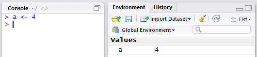
subsequent computations. For example, we could assign the variable a
the value 4. The command to do this is a < -4.
In that command we use the two character symbol
<- to mean "gets the value of" or "is assigned the value of".
When we enter the command a <- 4 and press the Enter
key, in RStudio, we should see the results as shown in Figure 1.
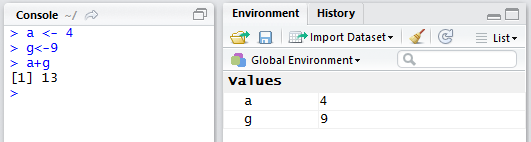
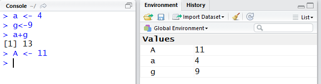
Let us continue with our example by defining another
variable, g and assigning it the value 9. The command to do
this is g<-9. Note that R understands this
even though we did not include extra spaces.
Feel free to add spaces in commands to make
those commands more readable!
Then we will form the expression a+g and press Enter.
All of this is shown in Figure 2.
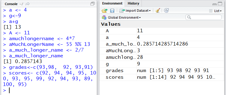
So far we have created and used two variables, a and g. That should raise a question in our minds: What are the legal names for variables? To start to answer that, let us look at another variable, namely, A. In Figure 3 we assign the value 11.
The important illustration in Figure 3 is that the variable A is distinct from the variable a. R is case-sensitive! This is a frequent cause of errors. Remember that variables that differ even by just the case (upper or lower) of one letter are different variables!
So far we have seen just single letter variables. The names of variables can be much longer than that. In Figure 4 we see such a longer name, amuchlongername.
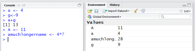
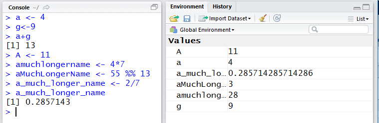
Variables should be given "meaningful" names. We can see that we can string together quite long names. However such names are a bit hard to read. There are at least two popular conventions that people use to make long names more readable. One is called "camelCase" where we start each internal different word in a variable name with an upper case letter. Thus, the camelCase alternative to our long variable name would be aMuchLongerName, a name that is much easier to read than was the previous version.
A second convention introduces the underscore character to separate words in the variable name. Such an alternative to our long variable name would be a_much_longer_name. There is a school of thought that this alternative should not be used in R. The foundation for that belief is that the precursor for R, namely S, actually used the underscore for the assignment operator. That use is no longer true in R so the objection seems to no longer hold. Just so that you know, many people use this style in their work.
Either convention makes it easier to read long names. In general, you should adopt one of these conventions and then stick to it; it is best not to mix conventions. Figure 5 demonstrates the two styles. Note that both are legal and that, of course, they produce distinct variables, as shown in the Environment pane.
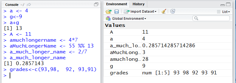
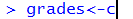
At this point we will look at assigning a variable a group of values. For this demonstration let us consider that we have a group of grades that we want to assign to a variable. The grades are 93, 98, 92, 93, and 91. In R-teminology, such a group is called a vector, that is, a vector is a collection of similar, probably related, values. The command to assign our vector to the variable grades is grades<-c(93,98,92,93,91) and this is shown in Figure 6.
 which says that we want to assign the variable grades
the vector created as we "combine" values, using the c
command which we then have to finish.
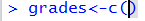
We continue by typing the left parenthesis and we find
that the system
supplies the
closing right parenthesis as shown in
which says that we want to assign the variable grades
the vector created as we "combine" values, using the c
command which we then have to finish.
We continue by typing the left parenthesis and we find
that the system
supplies the
closing right parenthesis as shown in
 .
Then, as we finish the command it looks like
.
Then, as we finish the command it looks like
 .
Then, even though the insertion pointer is inside the parentheses, we can
press Enter and the system will recognize this as the full command.
.
Then, even though the insertion pointer is inside the parentheses, we can
press Enter and the system will recognize this as the full command.
There are a few things to note in Figure 6.
First, there is no problem adding spaces in the command.
Second, because this is an assignment of a value
(in this case a vector of values)
to a variable, R Console just accepts the
command and prompts us for the next command.
Third, the RStudio Environment pane
shows  .
This gives us the name of the variable, the
kind of values in the vector (in this case,
the values are of type num),
the number of items in it (in this case, items indexed from 1 to 5),
and then we see the first number of values that are in the vector.
.
This gives us the name of the variable, the
kind of values in the vector (in this case,
the values are of type num),
the number of items in it (in this case, items indexed from 1 to 5),
and then we see the first number of values that are in the vector.
Let us create a larger vector to hold the scores shown in the following table:
| position | 1 | 2 | 3 | 4 | 5 | 6 | 7 | 8 | 9 | 10 | 11 | 12 | 13 | 14 |
| value | 92 | 94 | 94 | 95 | 100 | 93 | 95 | 99 | 92 | 94 | 93 | 89 | 100 | 95 |
 Second, in the Environment pane, we only get to see
the first five values in the vector, although the
system indicates that there are more values by ending the display line with an
ellipsis, the three dots, (...):
Second, in the Environment pane, we only get to see
the first five values in the vector, although the
system indicates that there are more values by ending the display line with an
ellipsis, the three dots, (...):

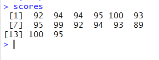
Since the last assignment statement in Figure 7 did not show us the values that are in scores let us just create the expression scores and press Enter. That is how we get the output given in Figure 8.
Let us finish this introductory page with just
a few examples of things that you can do with R.
For example, even though RStudio showed us,
back in Figure 7, that there are 14 items in scores,
and even though we could count the items in scores
and determine that there are indeed 14 items in that vector,
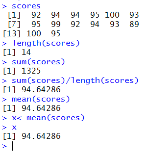
we can ask R directly for the length of the vector scores.
We do this with the command length(scores).
That command is shown as
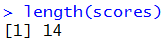 .
.
Or we can ask R to find the sum of
all the numbers in scores
by issuing the command
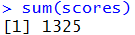 .
.
Of course, we could put these two together to come up
with the command
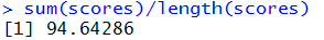 which really computes the average, known as the mean
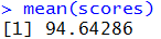
of the values in scores. As you might have guessed, R
has a single statement that computes the mean, namely, mean(),
which we illustrate as
which really computes the average, known as the mean
of the values in scores. As you might have guessed, R
has a single statement that computes the mean, namely, mean(),
which we illustrate as
An alternative to that would be to do the computation and
assign it to a variable. Then we could just use the variable name
as an expression to
display the computed average, as in
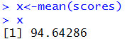 In fact, all of this was done and it is presented in Figure 9.
The only thing left to do for this web page is to quit R. We do that with the q() command, as shown in Figure 10.
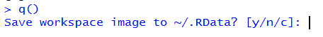
In all fairness, we should have talked about what R
meant with the question
 .
However, we will save that discussion for a different web page,
the working directory.
.
However, we will save that discussion for a different web page,
the working directory.
©Roger M. Palay
Saline, MI 48176 October, 2015