Mean

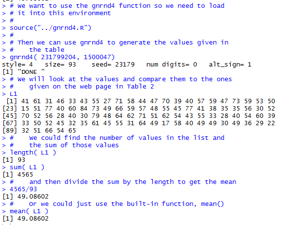
Now, let us see if we can do the same thing using R. In Figure 1 we see the Console pane of a R session, started from a directory where we had already loaded the gnrnd4() function. The first command in that pane performs the gnrnd4() just as we had specified above. Then, using the expression L1 we have R show us the entire collection of values. We can use this to confirm that this collection is identical to the one reported in Table 2.

Figure 1

Continuing in Figure 1, just to mimic our earlier actions, we ask R for the length of L1, that is, for the number of values in L1. R indicates that there 93 values. Then we ask R for the sum of those values, and we find that the sum is 4564. Then our next command is to find the quotient 4565/93, which R gives to us as 49.08602, the same value that we found above. Clearly, once we know that we can use mean() to find the mean of a collection of values we do not really need to find either the length or the sum of that collection. We did that just to follow along with our earlier actions.

Remember that we are looking at the mean as a measure of central tendency. That is, we are looking at this computed value to be representative of the "center" of the data. In the case of the values shown in table 2 our computed mean, 49.08602 really does seem to characterize the "center" of all 93 of those values.

We often say that the mean is a measure that is influenced by extreme values. Let us see what that means. What if we had been entering the values of Table 2 by hand and we made a simple error when we were typing item number 52. The value of the 52^nd item is 48. What if we had typed, in error, the value 4864. That would have been an extreme value in the sense that it is way larger than any of the other values in our collection. What would such an error do to the mean value?

To see what would happen we have the commands shown in Figure 2. We use the command L1[52] to get R to display the contents of the 52^nd item, and that item is shown to be 48. Then we use the command L1[52] <-4864 to change the value of that 52^nd item. We use the name of the collection, L1, to get R to display the entire collection of values. And, sure enough, we now have 4864 in position 52. Finally, we ask R to compute a new mean for the collection by giving the command mean(L1). The mean of this altered collection is now 100.871, vastly different from the old mean.

Figure 2

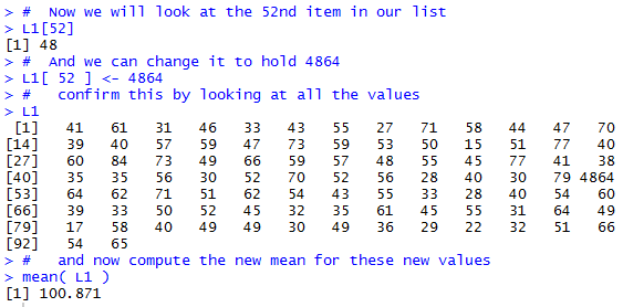
What we saw happening in Figure 2 was the introduction of a really extreme value. The result of doing so is a dramatic shift in the value of the mean. The mean is highly susceptible to having an extreme value.

In a more practical example, we might be looking at the mean income of WCC full time faculty. There are around 200 such people and their income, from all sources, is not at all identical but the values are not hugely different across the entire collection. However, if we were to have a new faculty member and if that faculty member were Bill Gates, then we would have a hugely different for the mean income of WCC full time faculty.

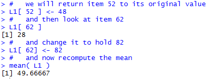
On the other hand, having slightly extreme values does not make such a huge difference. Consider the changes shown in Figure 3. First, we confirm, using L1[52], the value that we introduced before as an extreme value. Then we reset that item to hold the value 48. Then we inspect the 62^nd item just to see that it is 28. What if we had made a simple transposition error in entering the data and had entered the value 82 instead of 28.That is a much larger value than it was supposed to be. Then, with that altered value, we look at the mean of the values in L1. That mean turns out to be 49.66667, larger than the old mean, but not dramatically so.

Figure 3

Another aspect of the mean, for a large collection of values, is that it is really hard to cause that mean to change dramatically. A small story should demonstrate this. At one time the mean age of WCC students was 28.6 years. Our then Vice-President felt, for whatever reason, that it was important to make WCC a "younger, more youthful place". He announced that he intended to attract more younger students and to do so such that his actions would bring the mean age of WCC students down to 24. At the time there were 11,234 WCC students. Let us examine the math behind this.

With 11,234 students, in order for the average age to be 28.6, we need the sum of the ages of the students divided by 11,234 to be 28.6. That is we have the equation

With a large population, in this case 11,234 students, adding even a large number (say 1000) of students just does not move the mean very much. [Notice that in reality, the age of any one student cannot be all that extreme. Following the Jurassic Park theme, if we could suddenly find 100 students each of whom was 200,000 years old, and we could enroll them in WCC, then the mean would move by more than just a little.]

Downloading the script class ages.R and then running that script gives another example of how hard it is to move the mean.

Median

When there are an odd number of values in the collection then there will be a middle item, and that middle item will be the median. In fact, if `n` is the number of items in the collection, then, in the sorted version of the collection, item number `(n+1)/2` will be the middle item, and the value of that middle item will be the median.

On the other hand, consider the case where there are an even number of values in the collection, as in Table 4.

If there are an even number of items in the collection then the median is defined to be the average of the two middle items. In fact, if there are `n` items and `n` is an even number, then the median will be the average of the items in the sorted version of the collection that are in position `n/2` and `n/2+1`. [Given the way I constructed the values in Table 4, it is most likely the case that the two middle values were different, and as a result, it is most likely that the median value is not even a value in the collection. It is just the midpoint between the two middle values.]

The example in Table 4 was designed so that we would have a small number of values and so that the values would be spread out. Consider the more common, though still quite small, example shown in Table 5.

In most but not all cases the two middle values in Table 5-sorted are the same value. In fact, looking at that table it is clear that many of the values are duplicated. It is not a wonder that the two middle values are found within a "pile" of values that are the same. If you reload this web page many times you will eventually find a case where the first of the two middle values is in one "pile" of values and the second of the two middle values is in another "pile" of values. Only in that case does applying our rule, average the two middle values, give us a median that is not one of the values in the table.

Now let us see how we can do the same thing in R. First we will need to generate the data values. Then, we will mimic what we did here just to see that it can be done. Figure 4 shows those R commands and the associated output. [The highlight in Figure 4 was added later.]

Figure 4

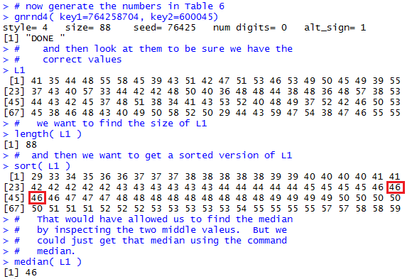
Generating and displaying the original data is as we have seen before. Figure 4 introduces a new function, namely sort() that is used to sort the values and then, since the result of the sort is not assigned to a variable, the result is displayed. This sorted collection is identical to the displayed values in Table 6-sorted. Based on the length of the data, 88, we know that we need to take the average of the 44^th and 45^th items in the sorted list. R conveniently gives us the first column of values telling us the index, the position, of the first data value in each row. Therefore we can identify those values in the second row. As an aid I highlighted those values in Figure 4.

All of the steps after generating the data were done to mimic what we did above. But the truth is we could have found the median by just telling R to find it for us. The command is median(L1) as shown in Figure 4, and the result is our expected 46.

Whereas the mean was highly influenced by extreme values, the median does not have this problem. Just think again about the situation where we were looking at the total annual income of full time WCC faculty. With about 200 such faculty we could certainly find the median value of that collection. Adding an extreme value, such as having Bill Gates join the faculty, would hardly change the median at all. Or, as a more specific example, Figure 4 showed us 88 values and we found the median of those 88 values to be 46, the average of 46 and 46. Go ahead and add, conceptually, an 89^th value. Make it as large as you want. Now you have 89 values and the median of those 89 values will be the one in position 45, and that is exactly 46. No change at all in the median!

Mode

So far, with the two earlier measures of central tendency, the mean and the median, we were able to find R commands, namely, mean() and median(), that simply compute the desired value. It would be nice if there were such a facility for finding the mode. Alas, if there is then I have not found it as part of the main R system.

Now we want to do the same thing in R. We start an R session, making sure that we do so such that gnrnd4() is already defined. Then we can generate the data using the given command. Following that we can even display the data, just to confirm that the R session is working with the same values that we saw in Table 8. And, finally, we can give the table(L1) command to have R generate the information that we saw in Table 8-tabulate. All of this appears in Figure 5.

Figure 5

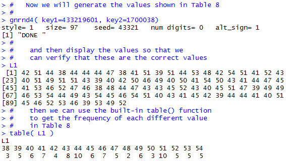
Now, just as we did "by hand" we can look at the values displayed by that table(L1) command, find the highest frequency value, then report the data value or values that are associated with that maximum frequency. Reading the final lines of Figure 5 we would say that the maximum frequency is 10 and that the data values 44 and 51 have that frequency. Therefore, the modal values are 44 and 51.

Of course, being a bit lazy, and probably a bit wise, we could ask R to help us find that maximum frequency and to make it easier to find all of the data values associated with it. One way to do this is to just sort the values. Figure 6 shows exactly that.

Figure 6

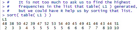
Having the table arranged as shown in Figure 6 makes it much easier for us to see the largest frequency (it is at the end of the output) and to identify all of the data values that have that frequency (they, too, are at the end of the output).

Actually, we could go a step or two further in using the power of R to find these values. Figure 7 demonstrates one approach to this. In that figure we start by storing the results of the table(L1) command into a new variable, t_hold. Then, we can just ask for the maximum value in t_hold. That will give us the maximum frequency of the items in L1. Then, we have R find the names, i.e., the data values, in t_hold, that have that frequency. This is done by using the command which(t_hold==10). [Note that == is the symbol for the test for equality.]

Figure 7

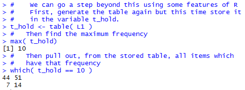
Indeed, in Figure 7 we see that our commands produced the maximum frequency and the two data values that are associated with that frequency. We have used the features of R to get the desired answer.

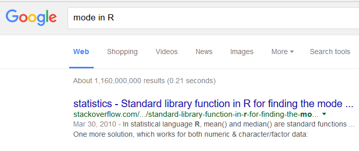
That would seem to be enough. R does not have a built-in function for finding the mode, but we did it anyway! However, the beauty of R is that there is a huge community of R users and just about anything that you want to do with R has been done by someone else before. Finding the mode surely seems like a simple and common task. Let us look for someone else's solution. I did a quick search on the web and found a link to Stackoverflow.com, shown in Figure 7.1, that seems to be exactly what I need.

Figure 7.1

Following that link took me to the following posting, shown in Figure 7.2:

Figure 7.2

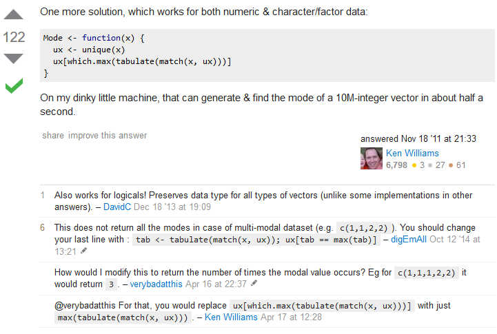
Using that suggestion from Ken Williams, and following up with some other suggestions, and then developing that into a function that I really would like to use in this course, brought me to develop the following script, given here in a form that you could copy from this web page and paste into either a R or a RStudio session.

Mode <- function(x, display=TRUE, na.rm = FALSE) {
  ## taken from a post by Ken Williams on Stackoverflow,
  ## and modified with other ideas and suggestions there,
  ## and then tuned by R. Palay for a speific use here.
  if(na.rm)
  {x = x[!is.na(x)]
  }
  ux <- unique(x)
  tab <- tabulate(match(x, ux))
  um <- max(tab)
  uy<-ux[tab == um]
  uy=sort(uy)
  if( display )
  {cat("Mode Frequency=",um,"Mode Value(s)=",uy,"\n")}
  c(um,uy)
}

Figure 8

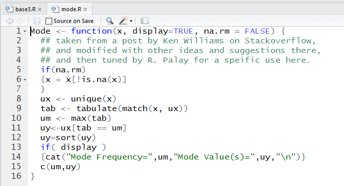
That script is now saved in the file mode.R on this web site. Therefore, you could right click on the link and then save the file to your machine, or you could right click on the link to base5.R to get a copy of the file shown in Figure 9.

Figure 9

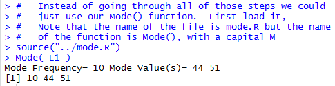
If you have done the latter then, if you use RStudio to open that file it will appear in the top left pane on your session. Once there you can highlight the desired command, as it was shown in Figure 9, and then click on the Run button at the top of that pane. That is how Figure 10 opens.

Figure 10

The second line of Figure 10 shows the call to our newly defined function Mode(). One important thing to notice here is that our new function is called Mode() with a capital M. Remember that R is case-sensitive; there is a difference between Mode() and mode(), the latter being a standard function of R that has nothing to do with finding the modal values of a collection of data.

When we call Mode(L1) the result is two lines of output, the first giving us the textual information and the second giving us three values, the first being the frequency of the mode and the remaining two values being the modal values that were found.

Recall that if we were to assign the function call to a variable, as in a <-Mode(L1), then the final value of the function is not displayed. We see this in the second call, a <-Mode(L1) which only produced the textual output.

If we then give the command a it actually produces the expected 3 values that were the final result of the function.

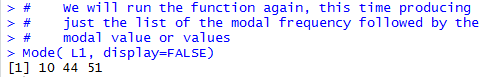
Still looking at Figure 10, a slightly more complex function call, b <-Mode(L1, display=FALSE) causes the textual output not to be produced, but the three result values are stored in the variable b.

Although we were able to find the mode of the data, just looking at the frequency table shows us that the values are rarely duplicated. However, if we look at the other two measures of central tendency we find that the