Using GNRND4

Return to Topics

This page describes the purpose of and the use of a set of routines encompassed in the file gnrnd4.R. The purpose and use are strictly related to the material of this course and in particular, to the coordination of data values on many of the web pages in this course and obtaining the same values in an R session.

There are many times when web pages in this course make reference to a collection of data values. For example, consider the
Now, although the particular web page may wish to talk about this data, it would be even better, and in the case of tests on web pages it may be highly desirable, if you could create a vector of the same values on your computer, and to do so in R.

If the web page is being displayed on a computer, then one possible solution would be to highlight the data in the table, copy it, and paste it to a file. Were we to do that then the file would have values in a number of rows and in a number of columns. R would have a hard time reading that directly, but we could manage it, with a lot of extra work. We would have to find some way to read that into R.

Another solution would be to copy the contents of the table and paste it into some program such as Microsoft Excel, where we could manipulate the data until we could write it to a file in a form that R could read.

Of course, neither of those solutions would be of any help if we were reading Table 1 on paper, as would be the case for a test. The obvious solution would be to just type the values into R. We have already seen the command to do this, namely:

But who wants to type that? In fact, I am sure that I couldn't type that without making at least one error! One interesting note here is that rather than being presented in table format if the values were presented as a comma separated list, such as we just saw in the command above, then we would have an easier time, using Excel, in converting them to a form that we could eventually read into R. But that still does not help in the printed version of the collection of values.

The values given in Table 1 above are generated, each time the page is loaded or refreshed, by a Javascript program that is part of this web page. In fact, if you were to use your browser to look at the page source then you would be able to find and read that Javascript program. The gnrnd4 solution to our challenge is just a function in R that performs exactly the same computations as did the Javascript program. Such a R function is provided in the file gnrnd4.R. The trick is

to get that file
to load it into R so that you can use it
to give the R function the starting point used by the Javascript program to generate the values.

There are a number of ways to achieve points 1 and 2. For one thing, you could download the file to your computer and then copy it into any R session that you are using. A second approach is just to use one R command during a session to both get and enter the gnrnd4.R commands into the R session. This latter approach requires you to have internet access but that should not be a problem for this course. Let us look at the performing this second method.

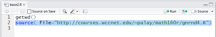
The command that we want to use is source(). In an R session, we will need to give the command source("http://courses.wccnet.edu/~palay/math160r/gnrnd4.R")

In order to ease your task of entering this long string, I have created a file, base2.R, that you can download by right clicking on this link to base2.R, and then using the "Save Link As..." option from your browser to put the file into the directory you want to use for this project. I have created a directory called project_02 in preparation for this task. I can now right click on the link above and get Figure 1

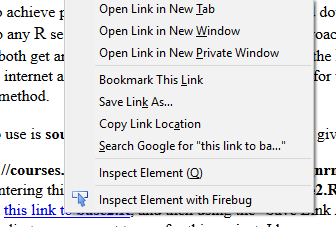
Select the "Save Link As..." option, and that opens the window Figure 2

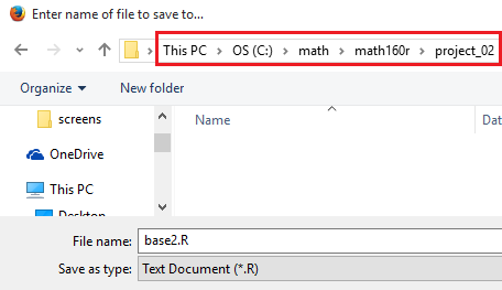
When the dialog box in Figure 2 opens it probably is not going to be pointing to our desired directory, but we can use that window to navigate to it. The image in Figure 2 shown here was captured when we were in the project_02 directory (highlighted by the red box in the figure). Once we have the directory selected we can just press the

button to save the file into that directory.

Figure 3 shows the directory after we have saved the file. Figure 3

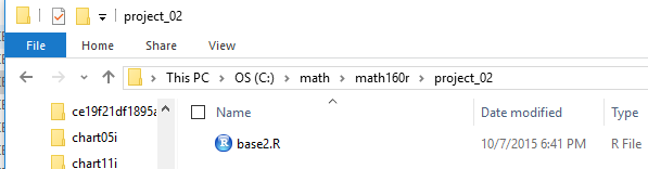
Now that we have the file in place, we can just double click on the file name and start RStudio.

When RStudio starts the Console pane shows the splash screen, the last few lines of which are captured in Figure 4. Figure 4

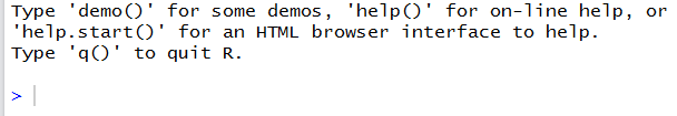
Note that there is no old workspace to load in this directory so R does not report loading any such workspace.

From Figure 5 we see that the top left pane of the RStudio screen shows the built-in editor and a display of the contents of the base2.R file. In particular, we see our desired command in that file. For Figure 5 we have highlighted that source() command. Figure 5

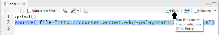
Then, we can have RStudio send that command to the Console pane and have R execute that command by clicking on the Run button, as shown in Figure 6. Figure 6

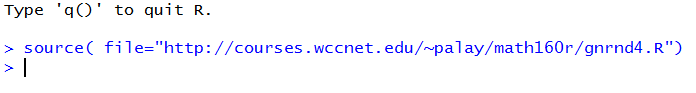
Indeed, Figure 7 shows the updated Console pane. There is not much to see there other than the fact that the command has been placed there and has been executed without any complaint. Figure 7

Whereas Figure 7 did not show evidence of any change, if we look at the Environment pane, shown in Figure 8, we see quite a change. Figure 8

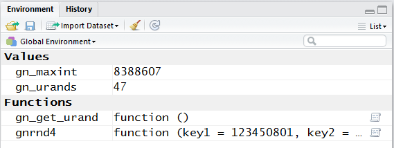
In particular, Figure 8 shows us that we now have two new variables defined, and two new functions that have been defined. Let us look at a demonstration of using the gnrnd4() function.

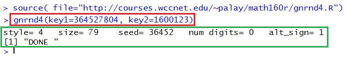
The line inside the red box in Figure 9 contains an instance of the gnrnd4() function. In that case we called the function with key1=364527804 and key2=1600123. Performing that command results in the displayed data inside the green box. That information is really not of much import at the moment. Figure 9

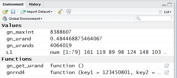
However, changes have been made. A look at Figure 10 shows, among other things, that there is now a new variable, L1 and that variable seems to be a list of 79 values, the first of which are 161, 119, 89, 98, 124, 148, and 103. Figure 10

We can actually see the entire collection of values in the Console screen by just giving R the name of the variable, L1. This is shown in Figure 11. Figure 11

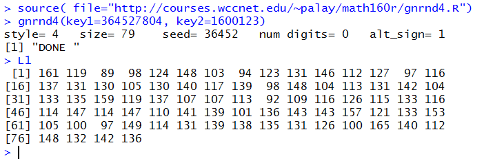
Note that the first column of values in Figure 11 gives us the numbering of the first element of L1 that is shown in that line. Thus, the first element is 161, the 16^th is 137, the 31^st is 133, the 46^th is 114, the 61^st is 105, and the 76^th is 148.

Probably the most interesting part of this is that knowing those key values I can produce the same values on this web page and display them in Table 2.

As noted above, the table here was produced from those key values, not from actually typing in the values.

Now we will quit R and tell it to save the workspace. Figure 12

Figure 13 shows us the project_02 directory. Because this was done on a PC, we can see the new "hidden" files that R has created. If we had done this on a Mac we could have used the "Unix" trick to show those same hidden files. Figure 13

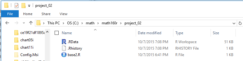
The fairly large size of the .RData file is due to the fact that the gnrnd4() function has been saved in that file as part of the workspace. As a result, if we were to restart RStudio (or, for that matter,R) from this directory, the gnrnd4() function will already be loaded and it will be ready to use.

One final note. Remember that the contents of Table 1 change every time this page is loaded or refreshed. I happened to have kept the key values that we used for this particular page, If you were to start RStudio, and if gnrnd4() has been loaded into your workspace, then you could produce and see a new L1 variable using the commands:

Return to Topics

©Roger M. Palay Saline, MI 48176 October, 2015