Two Samples: σ unknown
Return to Topics page
Before we start, we should recognize that the situation
described here is quite common, unlike the situation of
the previous page. There,
on the previous page,
we knew the standard deviation of the two populations.
Here we do not know those values.
Instead, we estimate the population standard deviations
by the sample standard deviations, s1
and s2.
There we knew that the distribution of the difference
of the sample means was normal with standard deviation
given by  .
Here we will use the value of
.
Here we will use the value of
 as the
standard deviation (the standard error) of the distribution
of the difference in the sample means. Furthermore,
that distribution will be a Student's t
distribution with a specific number of degrees of freedom.
We will see a "quick and dirty" way to get the degrees of
freedom and we will see a complex computation of the degrees of freedom.
The two methods give slightly different values. The former is much easier to compute
but it is not quite as "helpful" as is the latter. Once we have the computer to do the
complex computation there is little reason to use the "quick and dirty"
method. However, it is part of the course so we will see it here.
as the
standard deviation (the standard error) of the distribution
of the difference in the sample means. Furthermore,
that distribution will be a Student's t
distribution with a specific number of degrees of freedom.
We will see a "quick and dirty" way to get the degrees of
freedom and we will see a complex computation of the degrees of freedom.
The two methods give slightly different values. The former is much easier to compute
but it is not quite as "helpful" as is the latter. Once we have the computer to do the
complex computation there is little reason to use the "quick and dirty"
method. However, it is part of the course so we will see it here.
Other than the change from normal to
Student's t distributon, along with the newly required use of the
degrees of freedom, the work here will be almost identical to that
of the previous page. In fact, we will use the same examples here that we found
there, here we will the sample standard deviations rather than the population standard deviations.
We will start with
- two independent, random samples
from two populations;
- probably of different sample sizes, though this is not a requirement;
- each sample should have at least 30 items in it, although if the
underlying population is normal then we can get away with smaller samples;
- we do not know the values of standard deviation for each population.
The two populations have unknown mean values, μ1
for the first and μ2 for the second.
Confidence interval for the difference
μ1 - μ2
We construct a confidence interval for the difference of the
two means in the same way that we constructed one for the the mean of a population.
That is, we need to know
- the desired level of the confidence interval,
- a point estimate for the difference of the means, and
- the standard deviation of the difference of
sample means when we know the size of the samples
- the number of degrees of freedom that we should use.
But we can do this.
- Specifying a level for the confidence interval is easy.
We will call it α, meaning that if we want a 95% confidence level then
α=0.05, the area outside of our interval so that we will have 95%
of the area inside the interval.
- If we have two samples then they have respective sample means
 and
and
 .
The best point estimate for
μ1 - μ2
is
.
The best point estimate for
μ1 - μ2
is  .
.
- The distribution of the "difference in sample means" for samples of
size n1 and n2
taken from populations that have means
μ1
and μ2
is Student's t distribution with mean
μ1 - μ2
and standard deviation
.
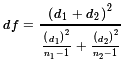
- The number of degrees of freedom can be computed first
using two intermediate values d1
and d2 computed as
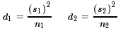 and then computing the degrees of freedom as
 To make this computation by hand is a royal pain.
To do it via the computer is almost trivial. Because it was such a pain,
the "quick and dirty"
common practice was to just use the smaller of
n1 - 1 and
n2 - 1 as the degrees of freedom.
(Remember that the higher the degrees of freedom the closer
Student's t is to approximating a normal distribution.
By using the smaller of the two values we are being
"conservative". That is, using that value we will get a confidence interval that is wider than
we really need it to be. Or, later, using this smaller value will make it harder
to reject a null hypothesis than is required by the given level of significance.)
To make this computation by hand is a royal pain.
To do it via the computer is almost trivial. Because it was such a pain,
the "quick and dirty"
common practice was to just use the smaller of
n1 - 1 and
n2 - 1 as the degrees of freedom.
(Remember that the higher the degrees of freedom the closer
Student's t is to approximating a normal distribution.
By using the smaller of the two values we are being
"conservative". That is, using that value we will get a confidence interval that is wider than
we really need it to be. Or, later, using this smaller value will make it harder
to reject a null hypothesis than is required by the given level of significance.)
All of that means that our confidence interval is given by
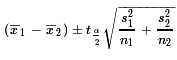 using the degrees of freedom that we either calculated or selected.
Now we are ready to walk through an example or two.
using the degrees of freedom that we either calculated or selected.
Now we are ready to walk through an example or two.
Case 1: We have two populations that are each normally distributed.
We want to create a 90% confidence interval for the difference of the means.
(Therefore, we want 5% of the area below the interval
and 5% of the area above the interval.)
We take samples of size n1 = 38
and n2 = 31, respectively.
Those samples yield sample means
 and
and
 .
Of course that means that
.
Of course that means that
 becomes
our point estimate.
becomes
our point estimate.
The samples also yield sample standard deviations,
s1 = 7.12
and
s2 = 6.13.
The standard deviation of the distribution of the difference of the
sample means for samples of the given sizes is
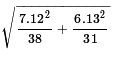 .
The value of that expression is about 1.5957.
All that remains is to find, for the standard Student's t distribution,
the value of t that has 5% of the area to the right of that value.
We could use the tables, a calculator, or the computer to find this.
However, no matter where we look for the value we also need a number
of degrees of freedom.
The "quick and dirty" method has us use the smaller of
38-1 and 31-1, or, rather, 30.
With 30 degrees of freedom we can determine that the t-value
that has 5% of the area to the right of that
t-value is approximately 1.697.
.
The value of that expression is about 1.5957.
All that remains is to find, for the standard Student's t distribution,
the value of t that has 5% of the area to the right of that value.
We could use the tables, a calculator, or the computer to find this.
However, no matter where we look for the value we also need a number
of degrees of freedom.
The "quick and dirty" method has us use the smaller of
38-1 and 31-1, or, rather, 30.
With 30 degrees of freedom we can determine that the t-value
that has 5% of the area to the right of that
t-value is approximately 1.697.
On the other hand, we could compute the more complex
degrees of freedom, finding
d1 = 7.12^2/38 ≈ 1.334
and
d2 = 6.13^2/31 ≈ 1.212
and that makes the degrees of freedom be
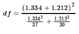 or
approximately 66.78369.
If we were using a table we would round this down to 66 degrees of
freedom. We find that the t-value with 66 degrees of freedom
that has 5% of the area to its right would be about 1.668.
We would find the same value if we used a calcualtor or computer to find
the t-value with 66 degrees of freedom although we would get more
digits displayed, as in 1.668271.
However, with a calulator or computer we can actually specify the
degrees of freedom as the value that we computed, the 66.78369.
Doing that gives the t-score of 1.667992
As you can see, this latter change is hardly noticable.
Therefore,depending upon how we got to the degrees of freedom
our confidence interval is:
or
approximately 66.78369.
If we were using a table we would round this down to 66 degrees of
freedom. We find that the t-value with 66 degrees of freedom
that has 5% of the area to its right would be about 1.668.
We would find the same value if we used a calcualtor or computer to find
the t-value with 66 degrees of freedom although we would get more
digits displayed, as in 1.668271.
However, with a calulator or computer we can actually specify the
degrees of freedom as the value that we computed, the 66.78369.
Doing that gives the t-score of 1.667992
As you can see, this latter change is hardly noticable.
Therefore,depending upon how we got to the degrees of freedom
our confidence interval is:
| Table 1 |
| using the 30 degrees of freedom from the "quick and dirty" rule |
using the 66 degrees of freedom from rounding the computed value down |
using the 66.78369 degrees of freedom from the computation |
1.8 ± 1.697*1.5957
1.8 ± 2.708
(-0.908, 4.508)
|
1.8 ± 1.668*1.5957
1.8 ± 2.662
(-0.862, 4.462)
|
1.8 ± 1.667992*1.5957
1.8 ± 2.6616
(-0.8616, 4.4616)
|
As you can see, the "quick and dirty" method produces a wider confidence interval
than does the computed method, and there is hardly any
difference between using the full computed degrees of freedom
or using that value rounded down to the next whole number.
Of course, we could perform all of those computations in R
by using the commands below. Please note that the style of the lines below is
to do the computations and put the
results into a variable and then display the value in the variable.
This means that there are many more lines than we need,
but this style also makes it easier to follow and
identify the results. Also, these lines include sections
for each of the three different values of the degrees of freedom,
corresponding to the three columns of Table 1 above.
n_one <- 38
n_two <- 31
s_one <- 7.12
s_two <- 6.13
d_one <- s_one^2/n_one
d_two <- s_two^2/n_two
std_err <- sqrt( d_one+d_two)
std_err
if( n_one < n_two)
{ df_simple <- n_one - 1} else
{ df_simple <- n_two - 1}
t_simple <- qt(0.05,df_simple,lower.tail=FALSE)
#simple, quick and dirty, t-score
t_simple
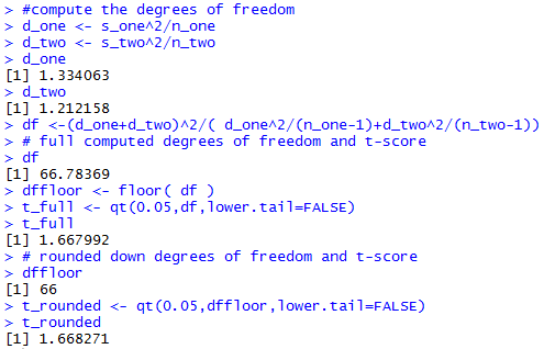
#compute the degrees of freedom
d_one <- s_one^2/n_one
d_two <- s_two^2/n_two
d_one
d_two
df <-(d_one+d_two)^2/( d_one^2/(n_one-1)+d_two^2/(n_two-1))
# full computed degrees of freedom and t-score
df
dffloor <- floor( df )
t_full <- qt(0.05,df,lower.tail=FALSE)
t_full
# rounded down degrees of freedom and t-score
dffloor
t_rounded <- qt(0.05,dffloor,lower.tail=FALSE)
t_rounded
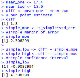
mean_one <- 17.4
mean_two <- 15.6
diff <- mean_one - mean_two
# our point estimate
diff
simple_moe <- t_simple*std_err
#simple margin of error
simple_moe
simple_low <- diff - simple_moe
simple_high<- diff + simple_moe
#simple confidence interval
simple_low
simple_high
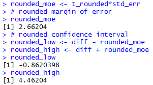
rounded_moe <- t_rounded*std_err
# rounded margin of error
rounded_moe
# rounded confidence interval
rounded_low <- diff - rounded_moe
rounded_high <- diff + rounded_moe
rounded_low
rounded_high
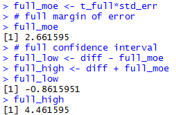
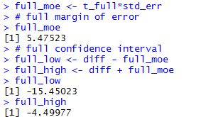
full_moe <- t_full*std_err
# full margin of error
full_moe
# full confidence interval
full_low <- diff - full_moe
full_high <- diff + full_moe
full_low
full_high
Those lines break into 5 sections:
The console result of those commands is given in Figure 1a
get the standard error and simple degrees of freedom,
get the calculated number of degrees of freedom,
get confidence interval for the simple case, get the confidence intercal
for the rounded case, and get the confidence interval for the
full case.
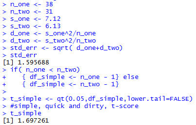
The console view of the commands to get the standard errror
and the simple degrees of freedom are
shown in Figure 1a.
Figure 1a
The console view of the commands to get the computed degrees of
freedom are
shown in Figure 1b.
Figure 1b
The console view of the commands to get the simple
confidence interval are
shown in Figure 1c.
Figure 1c
The console view of the commands to get the rounded
confidence interval are
shown in Figure 1d.
Figure 1d
The console view of the commands to get the full
confidence interval are
shown in Figure 1e.
Figure 1e
All of that work in R confirms the numbers shown in
Table 1 above.
Natuarlly, in any problem you will be told if you are to use
the simple method or the computed method. For your own work, since you
now have access to R, you might as well use the computed
method. It gives a higher value for the degrees of freedom and that results
in a lower t-value which, in turn, gives a lower value for
the margin of error, which makes the confidence interval
narrower.
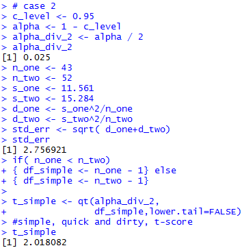
Case 2: We have two populations that are each normally distributed.
We want to create a 95% confidence interval for the difference of the means.
(Therefore we want 2.5% of the area below the interval and 2.5% of the area above the interval.)
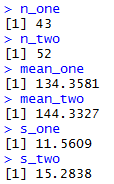
We take samples of size n1 = 43
and n2 = 52, respectively.
Those samples are given in Table 2 and Table 3 below.
We really have all the values that we need now,
the sample sizes, the sample means, the sample standard
deviations, and the confidence level.
We could just plug those values into the statements that we used above
and, from them, get the confidence interval.
The console view of the commands to get the standard errror
and the simple degrees of freedom are
shown in Figure 2a.
Figure 2a
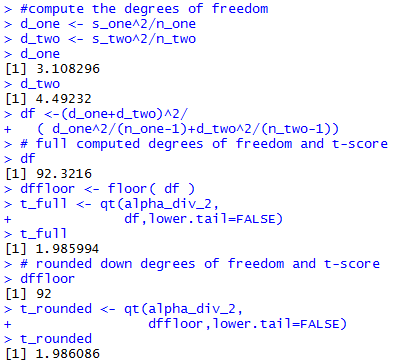
The console view of the commands to get the computed degrees of
freedom are
shown in Figure 2b.
Figure 2b
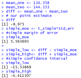
The console view of the commands to get the simple
confidence interval are
shown in Figure 2c.
Figure 2c
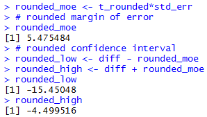
The console view of the commands to get the rounded
confidence interval are
shown in Figure 2d.
Figure 2d
The console view of the commands to get the full
confidence interval are
shown in Figure 2e.
Figure 2e
The result is that we have three versions of a 95% confidence interval:
- (-15.626,-4.324)
rounded to 3 decimal places, using the simple method,
- (-15.450,-4.500)
rounded to 3 decimal places, using the rounded method, and
- (-15.450,-4.500)
rounded to 3 decimal places, using the full method.
Of course, we used the sample mean values that this page supplied.
If those had not been given, then we would have to calculate
them. We could do this with the commands
gnrnd4( key1=1840954204, key2=0012801348 )
L_one <- L1
L_one
gnrnd4( key1=1481765104, key2=0015301435 )
L_two <- L1
L_two
n_one <- length(L_one)
n_two <- length(L_two)
s_one <- sd( L_one )
s_two <- sd( L_two )
mean_one <- mean( L_one )
mean_two <- mean( L_two )
n_one
n_two
mean_one
mean_two
s_one
s_two
the console view of the last
6 lines of which appears in Figure 3.
Figure 3
Then we could follow that with the more standard commands
that we used above
to produce the results shown in Figures 2a through 2e.
It does seem that this would be a good time to capture this
process in a function.
Consider the function ci_2unknown() shown below.
ci_2unknown <- function (
  s_one, n_one, x_one,
  s_two, n_two, x_two,
  cl=0.95)
{
    # try to avoid some common errors
    if( (cl <=0) | (cl>=1) )
      {return("Confidence interval must be strictly between 0.0 and 1")
      }
    if( (s_one <= 0)  | (s_two <= 0) )
      {return("Sample standard deviation must be positive")}
    if( (as.integer(n_one) != n_one ) |
        (as.integer(n_two) != n_two ) )
      {return("Sample size must be a whole number")}

    alpha <- 1 - cl
    alpha_div_2 <- alpha / 2

    d_one <- s_one^2/n_one
    d_two <- s_two^2/n_two
    std_err <- sqrt( d_one+d_two )

    if( n_one < n_two)
       { df_simple <- n_one - 1} else
       { df_simple <- n_two - 1}

    t_simple <- qt(alpha_div_2,
                   df_simple,lower.tail=FALSE)

    #compute the degrees of freedom
    d_one <- s_one^2/n_one
    d_two <- s_two^2/n_two

    df <-(d_one+d_two)^2/
         ( d_one^2/(n_one-1)+d_two^2/(n_two-1))

    t_full <- qt(alpha_div_2,
                 df,lower.tail=FALSE)

    diff <- x_one - x_two
    # our point estimate

    simple_moe <- t_simple*std_err

    simple_low <- diff - simple_moe
    simple_high<- diff + simple_moe

    full_moe <- t_full*std_err

    full_low <- diff - full_moe
    full_high <- diff + full_moe

    result <- c(full_low, full_high, full_moe,
                simple_low, simple_high, simple_moe,
                std_err,  alpha_div_2,  df, t_full,
                df_simple, t_simple, diff )

    names(result)<-c("Full Low", "Full High", "Full MOE",
                     "Simp Low", "Simp High", "Simp MOE",
                     "St. Error", "alpha/2","DF calc",
                     "t calc", "DF Simp", "t Simp", "Diff")
    return( result )
}
This function takes care of all of our work.
Figure 5 demonstrates the use of the function,
using the values that we have for Case:1,
via the two statements
source("../ci_2unknown.R")
ci_2unknown(7.12, 38, 17.4,
            6.13, 31, 15.6, 0.90 )
the first of which merely loads the function [we would have had to
place the file ci_2unknown.R into the parent directory (folder)
prior to doing this].
Figure 4
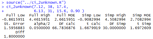
It is worth confirming that these are the same values that
we found in Figure 1a through Figure 1e above (although
the function does not report the values for the "rounded"
number of degrees of freedom.
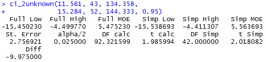
As another example we will call the function
with the input values for Case: 2. The function
is called via
ci_2unknown(11.561, 43, 134.358,
            15.284, 52, 144.333, 0.95)
and the console output is shown in Figure 5.
Figure 5
One of the problems associated with the command of Figure 5
is that it required us to re-type the some of the arguments.
With a little bit of preplanning,
we could have accomplished the same thing via
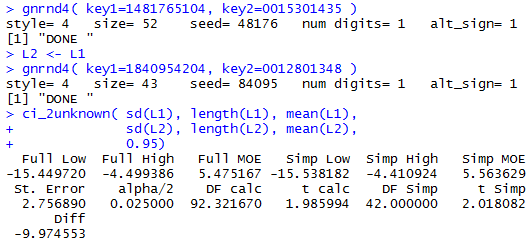
gnrnd4( key1=1481765104, key2=0015301435 )
L2 <- L1
gnrnd4( key1=1840954204, key2=0012801348 )
ci_2unknown( sd(L1), length(L1), mean(L1),
             sd(L2), length(L2), mean(L2),
             0.95)
Note that we have generated the second list first and then
we copied that list of values to the new variable L2.
We need to do that because gnrnd4() always
overwrites the values in L1.
The result of the four statement sequence in shown in Figure 6.
Figure 6
Rather than go through another example, Table 4
gives you the data that you need to do 5 more problems.
In fact, each time you reload the page you will get
5 new problems. Following Table 4 you will find the related answers
in Table 5.
(Please note that the algorithm used on this web page to
compute t-values is not as accurate as is the one used in R.
Therefore, the Full values in Table 5 might be slightly
off from the results that you get using R. The difference,
other than the usual rounding difference, should not be more than 0.001
in most cases.)
Because the cases presented in the tables above are dynamic I cannot
provide screen shots of getting those resuts in R.
You should be able to do these computation
and get approximately the same results.
The interpretion of a confidence interval is unchanged.
In Case 7 above, the Full confidence interval is
Hypothesis Testing for the difference of two means
We are in the usual situation where we do not know
the standard deviation of both populations.
Instead of building a confidence interval we want to
test the null hypothesis that the means
of the populations are identical.
That is, we have
H0: μ1 = μ2.
We take note here that we could restate the
null hypothesis as
H0: μ1 - μ2 = 0.
Using this form of the hypothesis is more convenient in that
it causes the distribution of sample means to be centered at 0.
To do this we need an alternative hypothesis, H1.
We have three possible alternatives and we choose
the one that is meaningful for the situation that arises.
Those three are:
| Initial Form | Restated version |
- H1: μ1 < μ2
a one-tail test
- H1: μ1 > μ2
a one-tail test
- H1: μ1 ≠ μ2
a two-tail test.
|
- H1: μ1 - μ2 < 0
a one-tail test
- H1: μ1 - μ2 > 0
a one-tail test
- H1: μ1 - μ2 ≠ 0
a two-tail test.
|
To perform a test
on
H0: μ1 - μ2 = 0
we need a test statistic.
That will be the
difference in the two sample means, namely,
.
We also need a level of significance for the test and
we need to know the distribution of the
difference in sample means. The level of significance
will be stated in the problem.
If the null hypothesis is true then the
distribution of the difference in the sample means is as above,
Student's t with mean 0 and standard deviation given by
. The
one additional issue is the degrees of freedom for that
Student's t distribution. Again,
we can use the "quick and dirty" by making the
degrees of freedom be one less than the smaller of the two sample sizes.
Alternatively, we can use the higher degrees of freedom
value that is the result of the strange
computation that we outlined above.
Recall that there is not a lot of difference in
the t-scores resulting from the two different methods. However,
there is some difference. It is possible that two samples would produce
results that would give enough evidence to reject H0
using the computed degrees of freedom but that the
same samples would not give enough evidence to reject H0
at the "quick and dirty" degrees of freedom.
In practice, since we have R and since we can do the required computation,
we will almost always use the computed value.
Case 8: Let us consider a specific example.
We have two populations.
We have
H0: μ1 = μ2
and our alternative hypothesis is
H1: μ1 < μ2.
Or, restated, we have
H0: μ1 - μ2 = 0
and our alternative hypothesis is
H1: μ1 - μ2 < 0.
We want to run the test with the level of significance set at
0.05. That is, even if the null hypothesis is true
we are willing to make a Type I error, incorrectly reject the null
hypothesis, 5% of the time.
We know that we are going to take samples of size 38
and 47, respectively.
The critical value approach:
We cannot move forward until we take the sample so that we can get
the two sample standard deviations.
Therefore, we will take our random samples (according to the given sample sizes)
and we find that
s1 = 3.48
and
s2 = 4.12.
These values yield a standard error of about 0.8245.
Then we can use 37 degrees of freedom if we apply the
"quick and dirty" approach, or we
can use 82.823 degrees of freedom derived from the computation outlined above.
The t-value for the standard
Student's t population with 37 degrees of freedom
that has 5% of the area to its left is about -1.687.
However the t-value for the standard
Student's t population with 82.823 degrees of freedom
that has 5% of the area to its left is about -1.663.
Our one-tail critical value is the t-score, -1.687 or
-1.663
times our standard error, 0.8245, below the
distribution mean. However, remember that under the null
hypothesis the distribution of the
difference in the sample means will have a mean of 0.
As a result, our critical value will be
-1.687*0.8245 ≈ -1.391 for the "quick and dirty"
method or -1.663*0.8245 ≈ -1.371 for the higher, computed,
degrees of freedom.
Therefore, if the difference between the means of our samples,
,
is less than the critical value, i.e., less than -1.391 for the "quick and dirty" approach,
or less than -1.371 for the "computed" or "full" approach,
then we will reject H0,
otherewise we will say that we have insufficient evidence to reject
the null hypothesis.
We took our two random samples, though we have not looked at their respecitve means.
It turns out that they have sample mean values of
25.46 and 26.91, respectively.
24.46 - 26.91 = -1.45 which is less
than either critical value.
Therefore, we reject H0 at the
0.05 level of significance.
Please note that if the difference of the sample means had been -1.38 then
we would have been rejected H0 using the
calculated degrees of freedom, but we would not have rejected it with the
"quick and dirty" degrees of freedom. This looks like more of an issue than
it is. The "gap" where this shows up is the values between -1.371 and -1.391.
The difference of the sample means could fall into this gap, but it is a small gap.
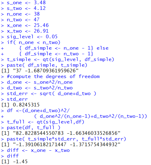
R statements, not necessarily the most
straightforward statements but rather statements that will
lead us to a function definiation later, for those computations are:
s_one <- 3.48
s_two <- 4.12
n_one <- 38
n_two <- 47
x_one <- 25.46
x_two <- 26.91
sig_level <- 0.05
if( n_one < n_two)
    { df_simple <- n_one - 1} else
    { df_simple <- n_two - 1}
t_simple <- qt(sig_level, df_simple)
paste( df_simple, t_simple)
#compute the degrees of freedom
d_one <- s_one^2/n_one
d_two <- s_two^2/n_two
std_err <- sqrt( d_one+d_two )
std_err
df <-(d_one+d_two)^2/
         ( d_one^2/(n_one-1)+d_two^2/(n_two-1))
t_full <- qt(sig_level,df)
paste(df, t_full )
paste( t_simple*std_err, t_full*std_err)
diff <- x_one - x_two
diff
The console view of those statements is given in Figure 7.
Figure 7
The attained significance approach:
For the attained significance approach we
still need to compute the standard error value
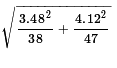 which we know is about 0.82453.
Then we take our two samples and get the sample means.
From those values we compute the difference,
24.46 - 26.91 = -1.45.
Because the null hypothesis has 0 as the value
of the difference of the true means, our question becomes
"What is the probability of getting a difference
of sample means such as we found or a larger difference?"
We "normalize" that difference by dividing it by the
standard error. That produces a t-value,
-1.45/0.8245 ≈ -1.759,
for
a standard normal distribution. As such we can use
a table, a calcualtor, or the computer to
find the probability of getting -1.759
or a value more negative than it.
That probability
depends upon the number of degrees of freedom.
For 37 degrees of freedom we find that
0.0434 is the attained significance.
For 82.823 degrees of freedom we find that
0.0412 is the attained significance.
We were running the test at
the 0.05 level of significance.
Our attained significance, no matter whether it was
0.0435 or 0.0412, is less than the 0.05 so we
reject H0.
which we know is about 0.82453.
Then we take our two samples and get the sample means.
From those values we compute the difference,
24.46 - 26.91 = -1.45.
Because the null hypothesis has 0 as the value
of the difference of the true means, our question becomes
"What is the probability of getting a difference
of sample means such as we found or a larger difference?"
We "normalize" that difference by dividing it by the
standard error. That produces a t-value,
-1.45/0.8245 ≈ -1.759,
for
a standard normal distribution. As such we can use
a table, a calcualtor, or the computer to
find the probability of getting -1.759
or a value more negative than it.
That probability
depends upon the number of degrees of freedom.
For 37 degrees of freedom we find that
0.0434 is the attained significance.
For 82.823 degrees of freedom we find that
0.0412 is the attained significance.
We were running the test at
the 0.05 level of significance.
Our attained significance, no matter whether it was
0.0435 or 0.0412, is less than the 0.05 so we
reject H0.
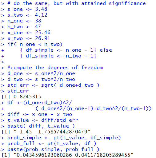
The R statements for those computations are:
# do the same, but with attained significance
s_one <- 3.48
s_two <- 4.12
n_one <- 38
n_two <- 47
x_one <- 25.46
x_two <- 26.91
if( n_one < n_two)
    { df_simple <- n_one - 1} else
    { df_simple <- n_two - 1}

#compute the degrees of freedom
d_one <- s_one^2/n_one
d_two <- s_two^2/n_two
std_err <- sqrt( d_one+d_two )
std_err
df <-(d_one+d_two)^2/
         ( d_one^2/(n_one-1)+d_two^2/(n_two-1))
diff <- x_one - x_two
t_value <- diff/std_err
paste( diff, t_value )
prob_simple <- pt(t_value, df_simple)
prob_full <- pt(t_value, df )
paste(prob_simple, prob_full )
The console view of those statements is given in Figure 8.
Figure 8
Case 9: Let us consider another example.
We have two populations.
We have
H0: μ1 = μ2
and our alternative hypothesis is
H1: μ1 ≠ μ2.
Or, restated, we have
H0: μ1 - μ2 = 0
and our alternative hypothesis is
H1: μ1 - μ2 ≠ 0.
We want to run the test with the level of significance set at
0.02. That is, even if the null hypothesis is true
we are willing to make a Type I error, incorrectly reject the null
hypothesis, 2% of the time.
We recognize that this is a two-tail test.
We will reject H0 if the difference
in the sample means is sufficiently far from 0 in either
the positive of negative direction.
Finally, we know that we are going to take samples of size 53
and 44, respectively.
The critical value approach:
We take our samples and find
s1 = 37.2
and
s2 = 35.1.
For the degrees of freedom we can use 43 or
we can compute a value from the sample standard deviations and the sample
sizes to get 93.415.
For 43 degrees of freedom the t-value with
1% of the area to its right is about 2.416.
Becasue the Student's t is symmetric, we know that the area to the
left of -2.416 is about 1%.
For 93.415 degrees of freedom the t-value with
1% of the area to its right is about 2.367.
Becasue the Student's t is symmetric, we know that the area to the
left of -2.367 is about 1%.
The standard deviation of the distribution of the
difference in sample means for samples of size 53 and
44, given the standard deviations of the samples
being 37.2 and 35.1 is
 which is about 7.356.
Our two-tail critical values are the low t-score,
either -2.416 or -2.367,
times our standard error, 7.356, below the
distribution mean, and the high
t-score, either 2.416 or 2.367, times our
standard error, 7.356 above the distribution mean.
However, remember that under the null
hypothesis the distribution of the
difference in the sample means will have a mean of 0.
As a result, using our "quick and dirty" degrees of freedom,
our critical values will be
-2.416*7.356 ≈ -17.774
and
2.416*7.356 ≈ 17.774.
On the other hand, using our computed degrees of freedom,
93.415,
our critical values will be
-2.367*7.356 ≈ -17.411
and
2.367*7.356 ≈ 17.411.
We took our random samples. Now we look at the sample means.
If the difference between the means,
,
is not between -17.774 and 17.774 in the former case, or
is not between -17.411 and 17.411 in the latter case
then we will reject H0,
otherewise we will say that we have insufficient evidence to reject
the null hypothesis.
It turns out that the sample means are
276.42 and 261.13, respectively.
276.42 - 261.13 = 15.29 which is between
either set of
the critical values.
Therefore, in either approach we do not reject H0 at the
0.02 level of significance.
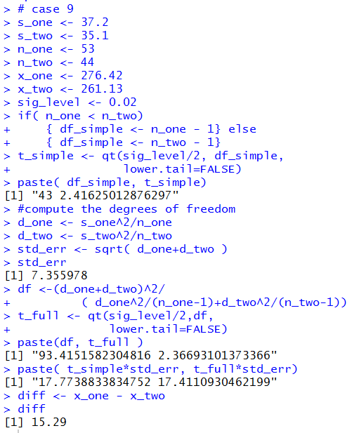
The R statements for those computations are:
# case 9
s_one <- 37.2
s_two <- 35.1
n_one <- 53
n_two <- 44
x_one <- 276.42
x_two <- 261.13
sig_level <- 0.02
if( n_one < n_two)
    { df_simple <- n_one - 1} else
    { df_simple <- n_two - 1}
t_simple <- qt(sig_level/2, df_simple,
               lower.tail=FALSE)
paste( df_simple, t_simple)
#compute the degrees of freedom
d_one <- s_one^2/n_one
d_two <- s_two^2/n_two
std_err <- sqrt( d_one+d_two )
std_err
df <-(d_one+d_two)^2/
         ( d_one^2/(n_one-1)+d_two^2/(n_two-1))
t_full <- qt(sig_level/2,df,
             lower.tail=FALSE)
paste(df, t_full )
paste( t_simple*std_err, t_full*std_err)
diff <- x_one - x_two
diff
The console view of those statements is given in Figure 9.
Figure 9
The attained significance approach:
With the given values of the population standard deviations and the
known sample sizes we compute the standard error as before,
namely, 7.356.
Then we take our samples and find the sample means,
276.42 and 261.13.
We note that the difference 276.42 - 261.13
will be positive. Therefore, we need to find the
probability of getting that value or higher from our
distribution which has mean 0 and standard deviation
7.356. We can do this with a pt()
function call. The result then needs to be multiplied by 2 because
we are looking at a two-tailed test. We are answering the
question "What is the probability of being that far away
from the mean, in either direction?" We calculated one side
so we need to double it to get the total probability.
The one-side value is 0.0188, so the total will be
0.0376, a value that is larger than our level of significance,
0.02, in the problem statement. Therefore, we do not reject H0
at the 0.02 level of significance.
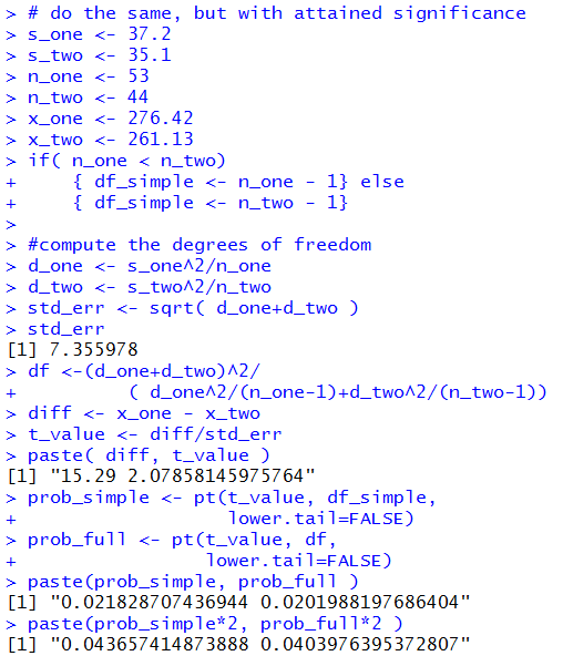
The following R statements do these computations:
# do the same, but with attained significance
s_one <- 37.2
s_two <- 35.1
n_one <- 53
n_two <- 44
x_one <- 276.42
x_two <- 261.13
if( n_one < n_two)
    { df_simple <- n_one - 1} else
    { df_simple <- n_two - 1}

#compute the degrees of freedom
d_one <- s_one^2/n_one
d_two <- s_two^2/n_two
std_err <- sqrt( d_one+d_two )
std_err
df <-(d_one+d_two)^2/
         ( d_one^2/(n_one-1)+d_two^2/(n_two-1))
diff <- x_one - x_two
t_value <- diff/std_err
paste( diff, t_value )
prob_simple <- pt(t_value, df_simple,
                  lower.tail=FALSE)
prob_full <- pt(t_value, df,
                lower.tail=FALSE)
paste(prob_simple, prob_full )
paste(prob_simple*2, prob_full*2 )
The console image of those statements is given in Figure 10.
Figure 10
At this point is seems appropriate to try to capture these
commands in a function so that we can use the function
to solve any problem like these.
Consider the following function definition:
hypoth_2test_unknown <- function(
  s_one, n_one, x_one,
  s_two, n_two, x_two,
  H1_type=0, sig_level=0.05)
{ # perform a hypothesis test for the difference of
  # two means when we do not know the standard deviations of
  # the two populations and the alternative hypothesis is
  #      !=  if H1_type==0
  #      <   if H1_type < 0
  #      >   if H1_type > 0
  # Do the test at sig_level significance.
  if( n_one < n_two)
    { df_simple <- n_one - 1} else
    { df_simple <- n_two - 1}
  use_sig_level = sig_level;
  if( H1_type == 0 )
    { use_sig_level = sig_level/2}
  t_simple <- -qt(use_sig_level, df_simple)

  #compute the degrees of freedom
  d_one <- s_one^2/n_one
  d_two <- s_two^2/n_two
  std_err <- sqrt( d_one+d_two )

  df <-(d_one+d_two)^2/
         ( d_one^2/(n_one-1)+d_two^2/(n_two-1))
  t_full <- -qt(use_sig_level,df)

  extreme_simple <-   t_simple*std_err
  extreme_full   <-   t_full * std_err

  diff <- x_one - x_two
  diff_standard <- diff / std_err

  decision_simple <- "Reject"
  decision_full   <- "Reject"
  if( H1_type < 0 )
     { crit_low_simple <-  - extreme_simple
       crit_high_simple <- "n.a."
       if( diff > crit_low_simple)
         { decision_simple <- "do not reject"}
       crit_low_full <-  - extreme_full
       crit_high_full <- "n.a."
       if( diff > crit_low_full)
         { decision_full <- "do not reject"}
       attained_simple <- pt( diff_standard, df_simple)
       attained_full   <- pt( diff_standard, df )
       alt <- "mu_1 < mu_2"
     }
  else if ( H1_type == 0)
     { crit_low_simple  <-  - extreme_simple
       crit_high_simple <-  extreme_simple
       if( (crit_low_simple < diff) &
           (diff < crit_high_simple) )
          { decision_simple <- "do not reject"}
       crit_low_full  <-  - extreme_full
       crit_high_full <-  extreme_full
       if( (crit_low_full < diff) &
           (diff < crit_high_full) )
          { decision_full <- "do not reject"}


       if( diff < 0 )
         { attained_simple <- 2*pt(diff_standard, df_simple)
           attained_full   <- 2*pt(diff_standard, df)
         }
       else
         { attained_simple <- 2*pt(diff_standard,
                             df_simple,
                             lower.tail=FALSE)
           attained_full   <- 2*pt(diff_standard,
                             df,
                             lower.tail=FALSE)

         }
       alt <- "mu_1 != mu_2"
     }
  else
     { crit_low_simple <- "n.a."
       crit_high_simple <-  extreme_simple
       if( diff < crit_high_simple)
         { decision_simple <- "do not reject"}
       crit_low_full <- "n.a."
       crit_high_full <-  extreme_full
       if( diff < crit_high_full)
         { decision_full <- "do not reject"}


       attained_simple <- pt(diff_standard, df_simple,
                         lower.tail=FALSE)
       attained_full <- pt(diff_standard, df,
                         lower.tail=FALSE)

       alt <- "mu_1 > mu_2"
     }
 result <- c( alt, s_one, n_one, x_one,
                   s_two, n_two, x_two,
                   std_err, diff, sig_level,
                   diff_standard, df,
                   crit_low_full, crit_high_full,
                   attained_full, decision_full,
                   df_simple,
                   crit_low_simple, crit_high_simple,
                   attained_simple, decision_simple
                   )
 names(result) <- c("H1:",
                    "s_one", "n_one","mean_one",
                    "s_two", "n_two","mean_two",
                    "std. err.", "difference", "sig level",
                    "t-value", "full df",
                    "full low", "full high",
                    "full Attnd", "full decision",
                    "simple df",
                    "simp low", "simp high",
                    "simp Attnd", "simp decision"
                    )
 return( result)

}
Once this function has been installed we can
accomplish the analysis of Case: 8 above via the command
hypoth_2test_unknown(3.48, 38, 25.46,
                     4.12, 47, 26.91, -1, 0.05)
Figure 11 shows the console view of that command.
Figure 11
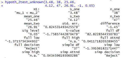
In a similar fashion, Case: 9 could have been
handles via
hypoth_2test_unknown(37.2, 53, 276.42,
                     35.1, 44, 261.13, 0, 0.02)
Figure 12 shows the console view of that command.
Figure 12
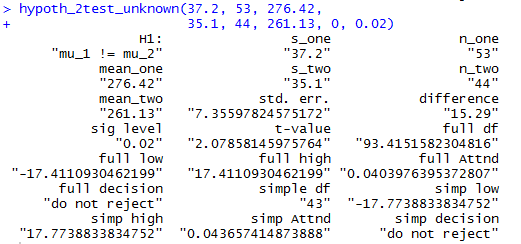
Clearly, the command shortens our work and still provides
us with all of the details.
Case 10: We can use the function in a new problem.
We start with two populations.
We know that the two populations have a normal distributon.
As such we can "get away with" having slightly smaller samples.
Our null hypothesis is that the means of the two populations is the same.
Thus, we have
H0: μ1 - μ2 = 0
and our alternative hypothesis is
H1: μ1 - μ2 > 0.
We want to test H0 at the
0.025 level of signifcance. (This is a one-tail test.)
We agree to take samples from each population, where the sample size is 24 and 28,
respectively.
Table 6 has the sample from the first population.
Table 7 has the sample from the second population.
For this information we need to do a little processing.
We want the sample size,
the sample mean, and the sample standard deviation for each of the two samples.
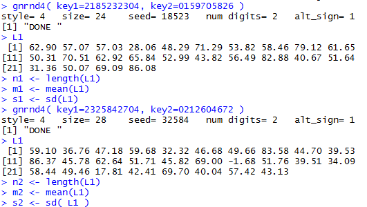
We can generate the data and get those values with the R commands:
gnrnd4( key1=2185232304, key2=0159705826 )
L1
n1 <- length(L1)
m1 <- mean(L1)
s1 <- sd(L1)
gnrnd4( key1=2325842704, key2=0212604672 )
L1
n2 <- length(L1)
m2 <- mean(L1)
s2 <- sd( L1 )
It was not necessary to display the data but it is nice to have
the display so that
we can confirm that we have correctly entered the
gnrnd4() comamnds. The console view follows in Figure 13.
Figure 13
Then,to do the problem we just need the command
hypoth_2test_unknown(s1, n1, m1,
                   s2, n2, m2,
                   1, 0.025)
That command produces the output of Figure 14.
Figure 14
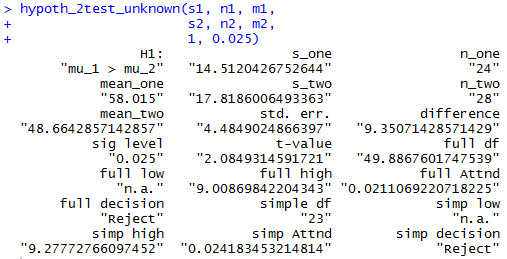
Figure 14 gives us the standard error, 4.485,
the two sample means, 58.015 and 48.664,
the two sample standard deviations, 14.512 and 17.819,
the difference of the means, 9.351,
the critical values, 9.009 for the computed degrees of freedom
and 9.278 for the "quick and dirty" degrees of freedom,
(there is only one for each method since this is a one-tail test),
the attained significance, 0.0211 and 0.0242 for the two methods,
and even the decision,
Reject in both situations.
We would reach that decision using the critical value approach because the
difference was greater than the critical value,
or by the attained significance approach because the attained significance
was less than the level of significance.
Return to Topics page
©Roger M. Palay
Saline, MI 48176 February, 2016