Two Samples: Sigma's known

Two Samples: σ known

Return to Topics page
Before we start, we should recognize that the situation described here almost never exists. How are we to know the standard deviation of two populations when we do not know their respective mean values? This situation is presented here, even though it would be strange to find it in real life (though not strange to find it on a stat test) because it is a straightforward computation that sets the pattern for the situations that will be presented in subsequent pages.

We will start with

two independent, random samples from two populations;
probably different sample sizes, though this is not a requirement;
each sample should have at least 30 items in it, although if the underlying populations are normal then we can get away with smaller samples.

There is nothing strange about those issues. However, for this presentation we will assume that we know one more thing.

We know the values of standard deviation for each population, σ₁ for the first population and σ₂ for the second.

The two populations have unknown mean values, μ₁ for the first and μ₂ for the second.

Confidence interval for the difference μ₁ - μ₂

We construct a confidence interval for the difference of the two means in the same way that we constructed one for the the mean of a population. That is, we need to know

the desired level of the confidence interval,
a point estimate for the difference of the means, and
the standard deviation of the difference of sample means when we know the size of the samples.

But we can do this.

Specifying a level for the confidence interval is easy. We will call it α, meaning that if we want a 95% confidence level then α=0.05, the area outside of our interval so that we will have 95% of the area inside the interval.
If we have two samples then they have respective sample means and . The best point estimate for μ₁ - μ₂ is .
The distribution of the "difference in sample means" for samples of size n₁ and n₂ taken from populations that have means μ₁ and μ₂ with standard deviations σ₁ and σ₂ is normal with mean μ₁ - μ₂ and standard deviation .

All of that means that our confidence interval is given by

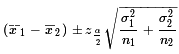
Now we are ready to walk through an example or two.

Case 1: We have two populations that are each normally distributed. We want to create a 90% confidence interval for the difference of the means. (Therefore, we want 5% of the area below the interval and 5% of the area above the interval.) We know that the standard deviation of the first is σ₁ = 7.4 and the standard deviation of the second is σ₂ = 6.2. We take samples of size n₁ = 38 and n₂ = 31, respectively. Those samples yield sample means

and

. Of course that means that

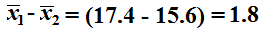becomes our point estimate. The standard deviation of the distribution of the difference of the sample means, for samples of the given sizes, is

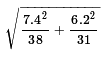. But the value of that expression is about 1.6374. All that remains is to find, for the standard normal distribution, the value of z that has 5% of the area to the right of that value. We could use the tables, a calculator, or the computer to find this. It turns out to be about 1.645. Therefore, our confidence interval is 1.8 ± 1.645*1.6374
1.8 ± 2.693
(^-0.893, 4.493) which leaves us with a margin of error of 2.693.

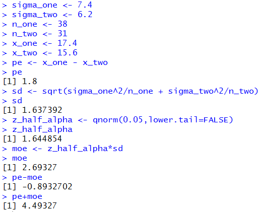
Of course, we could perform all of those computations in R by using the commands
sigma_one <- 7.4 sigma_two <- 6.2 n_one <- 38 n_two <- 31 x_one <- 17.4 x_two <- 15.6 pe <- x_one - x_two pe sd <- sqrt(sigma_one^2/n_one + sigma_two^2/n_two) sd z_half_alpha <- qnorm(0.05,lower.tail=FALSE) z_half_alpha moe <- z_half_alpha*sd moe pe-moe pe+moe
The console result of those commands is given in Figure 1.

Figure 1

Case 2: We have two populations that are each normally distributed. We want to create a 95% confidence interval for the difference of the means. (Therefore we want 2.5% of the area below the interval and 2.5% of the area above the interval.) We know that the standard deviation of the first is σ₁ = 12.8 and the standard deviation of the second is σ₂ = 15.3. We take samples of size n₁ = 43 and n₂ = 52, respectively. Those samples are given in Table 1 and Table 2 below.

We really have all the values that we need now, the known σ's, the sample sizes, the sample means, and the confidence level. We could just plug those values into the statements that we used above and, from them, get the confidence interval. Figure 2 shows the console view of such statements.

Figure 2

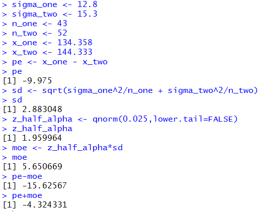
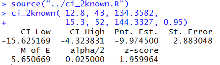
The result is that we have a 95% confidence interval: (-15.626,-4.324) rounded to 3 decimal places.

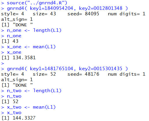
Of course, we used the sample mean values that this page supplied. If those had not been given, then we would have to calculate them. We could do this with the commands
source("../gnrnd4.R") gnrnd4( key1=1840954204, key2=0012801348 ) n_one <- length(L1) n_one x_one <- mean(L1) x_one gnrnd4( key1=1481765104, key2=0015301435 ) n_two <- length(L1) n_two x_two <- mean(L1) x_two
the console view of which appears in Figure 3.

Figure 3

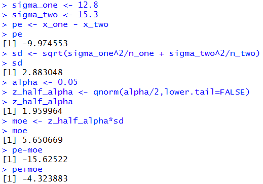
Then we could follow that with the more standard commands
sigma_one <- 12.8 sigma_two <- 15.3 pe <- x_one - x_two pe sd <- sqrt(sigma_one^2/n_one + sigma_two^2/n_two) sd alpha <- 0.05 z_half_alpha <- qnorm(alpha/2,lower.tail=FALSE) z_half_alpha moe <- z_half_alpha*sd moe pe-moe pe+moe
to produce the results in Figure 4.

Figure 4

It does seem that this would be a good time to capture this process in a function. Consider the function ci_2known() shown below.
ci_2known <- function ( sigma_one, n_one, x_one, sigma_two, n_two, x_two, cl=0.95) { # try to avoid some common errors if( (cl <=0) | (cl>=1) ) {return("Confidence interval must be strictly between 0.0 and 1") } if( (sigma_one <= 0) | (sigma_two <= 0) ) {return("Population standard deviation must be positive")} if( (as.integer(n_one) != n_one ) | (as.integer(n_two) != n_two ) ) {return("Sample size must be a whole number")} pe <- x_one - x_two sd <- sqrt(sigma_one^2/n_one + sigma_two^2/n_two) alpha <- 1-cl z_half_alpha <- qnorm(alpha/2,lower.tail=FALSE) moe <- z_half_alpha*sd low_end <- pe-moe high_end <- pe+moe result <- c(low_end, high_end, pe, sd, moe, alpha/2, z_half_alpha) names(result)<-c("CI Low","CI High","Pnt. Est.", "St. Error", "M of E", "alpha/2","z-score") return( result ) }
This function takes care of all of our work. Figure 5 demonstrates the use of the function, using the values that we have for Case:2, via the two statements
source("../ci_2known.R") ci_2known( 12.8, 43, 134.3582, 15.3, 52, 144.3327, 0.95)
the first of which merely loads the function [we would have had to place the file ci_2known.R into the parent directory (folder) prior to doing this].

Figure 5

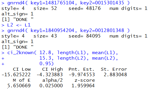
One of the problems associated with the command of Figure 5 is that it required us to re-type some of the arguments. With a little bit of preplanning, we could have accomplished the same thing via
gnrnd4( key1=1481765104, key2=0015301435 ) L2 <- L1 gnrnd4( key1=1840954204, key2=0012801348 ) ci_2known( 12.8, length(L1), mean(L1), 15.3, length(L2), mean(L2), 0.95)
Note that we have generated the second list first and then we copied that list of values to the new variable L2. We need to do that because gnrnd4() always overwrites the values in L1. The result of the four statement sequence in shown in Figure 6.

Figure 6

Rather than go through another example, Table 3 gives you the data that you need to do 5 more problems. In fact, each time you reload the page you will get 5 new problems. Following Table 3 you will find the related answers in Table 4. Because the cases presented in the tables above are dynamic I cannot provide screenshots of getting those results in R. You should be able to do these computations and get approximately the same results.

The interpretation of a confidence interval is unchanged. In Case 7 above, the confidence interval is

Hypothesis Testing for the difference of two means

Remember, we are still in a situation where we know, by some miracle, the standard deviation of both populations. Instead of building a confidence interval we want to test the null hypothesis that the means of the populations are identical. That is, we have H₀: μ₁ = μ₂. We take note here that we could restate the null hypothesis as H₀: μ₁ - μ₂ = 0. Using this form of the hypothesis is more convenient in that it causes the distribution of sample means to be centered at 0.

To do this we need an alternative hypothesis, H₁. We have three possible alternatives and we choose the one that is meaningful for the situation that arises. Those three are:

Initial Form	Restated version
H₁: μ₁ < μ₂ a one-tail test H₁: μ₁ > μ₂ a one-tail test H₁: μ₁ ≠ μ₂ a two-tail test.	H₁: μ₁ - μ₂ < 0 a one-tail test H₁: μ₁ - μ₂ > 0 a one-tail test H₁: μ₁ - μ₂ ≠ 0 a two-tail test.

To perform a test on H₀: μ₁ - μ₂ = 0 we need a test statistic. That will be the difference in the two sample means, namely,

. We also need a level of significance for the test and we need to know the distribution of the difference in sample means. The level of significance will be stated in the problem. If the null hypothesis is true then the distribution of the difference in the sample means is as above, normal with mean 0 and standard deviation given by

.

Case 8: Let us consider a specific example. We have two populations and we know that σ₁ = 3.48 and σ₂ = 4.12. We have H₀: μ₁ = μ₂ and our alternative hypothesis is H₁: μ₁ < μ₂. Or, restated, we have H₀: μ₁ - μ₂ = 0 and our alternative hypothesis is H₁: μ₁ - μ₂ < 0. We want to run the test with the level of significance set at 0.05. That is, even if the null hypothesis is true we are willing to make a Type I error, incorrectly reject the null hypothesis, 5% of the time. We know that we are going to take samples of size 38 and 47, respectively.

The critical value approach:

The z-value for the standard normal population that has 5% of the area to its left is about -1.645. The standard deviation of the distribution of the difference in sample means for samples of size 38 and 47, given the standard deviations of the populations being 3.48 and 4.12 is

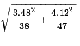which is about 0.82453. Our one-tail critical value is the z-score, -1.645, times our standard error, 0.82453, below the distribution mean. However, remember that under the null hypothesis the distribution of the difference in the sample means will have a mean of 0. As a result, our critical value will be -1.645*0.82453 ≈ -1.356. Therefore, we will take our random samples (according to the given sample sizes) and if the difference between the means,

, is less than the critical value, i.e., less than -1.356, then we will reject H₀, otherwise we will say that we have insufficient evidence to reject the null hypothesis.

We take our two random samples. They have sample mean values of 25.46 and 26.91, respectively. 24.46 - 26.91 = -1.45 which is less than the critical value. Therefore, we reject H₀ at the 0.05 level of significance.

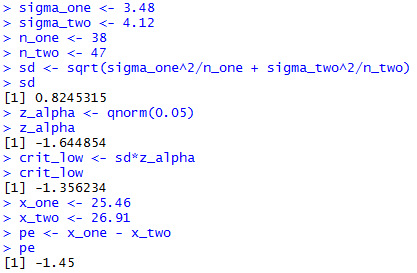
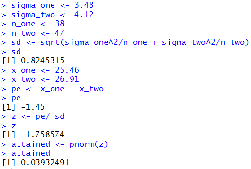
The R statements for those computations are:
sigma_one <- 3.48 sigma_two <- 4.12 n_one <- 38 n_two <- 47 sd <- sqrt(sigma_one^2/n_one + sigma_two^2/n_two) sd z_alpha <- qnorm(0.05) z_alpha crit_low <- sd*z_alpha crit_low x_one <- 25.46 x_two <- 26.91 pe <- x_one - x_two pe
The console view of those statements is given in Figure 7.

Figure 7

The attained significance approach:

For the attained significance approach we still need to compute the standard error value

which we know is about 0.82453. Then we take our two samples and get the sample means. From those values we compute the difference, 24.46 - 26.91 = -1.45. Because the null hypothesis has 0 as the value of the difference of the true means, our question becomes "What is the probability of getting a difference of sample means such as we found or a larger difference?" We "normalize" that difference by dividing it by the standard error. That produces a z-value, -1.45/0.82453 ≈ -1.759, for a standard normal distribution. As such we can use a table, a calculator, or the computer to find the probability of getting -1.759 or a value more negative than it. That probability, 0.0393, is the attained significance. We were running the test at the 0.05 level of significance. Our attained significance 0.0393 is less than the 0.05 so we reject H₀.

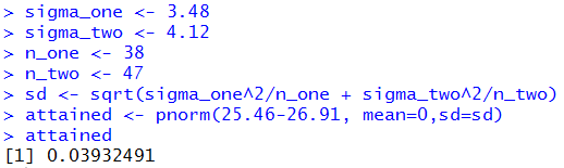
The R statements for those computations are:
sigma_one <- 3.48 sigma_two <- 4.12 n_one <- 38 n_two <- 47 sd <- sqrt(sigma_one^2/n_one + sigma_two^2/n_two) sd x_one <- 25.46 x_two <- 26.91 pe <- x_one - x_two pe z <- pe/ sd z attained <- pnorm(z) attained
The console view of those statements is given in Figure 8.

Figure 8

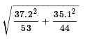
Just for the record, the computation of Figure 8 did not need to be so extensive. Recall that the pnorm() function allows us to specify the mean and standard deviation rather than forcing us to compute the "normalized" value of z. Also, we can enter the difference of the means as the raw difference. The statements shown in Figure 9 employ these techniques.

Figure 9

One seemingly strange part of Figure 9, the use of sd=sd, deserves some additional comment. The name of the parameter in the pnorm() function is sd, just as the parameter for the mean is mean. We need to assign a value to that parameter. A structure such as sd=3.12 would tell pnorm() to use that value for the standard deviation. Prior to the use of pnorm() in Figure 9 we defined a variable, sd to hold the computed standard error. It did not need to be called sd but there is no harm in using that name. Thus, the structure sd=sd tells pnorm() to assign the value stored in the variable sd, the one on the right of the equal sign, to the parameter sd, the one on the left of the equal sign.

Case 9: Let us consider another example. We have two populations and we know that σ₁ = 37.2 and σ₂ = 35.1. We have H₀: μ₁ = μ₂ and our alternative hypothesis is H₁: μ₁ ≠ μ₂. Or, restated, we have H₀: μ₁ - μ₂ = 0 and our alternative hypothesis is H₁: μ₁ - μ₂ ≠ 0. We want to run the test with the level of significance set at 0.02. That is, even if the null hypothesis is true we are willing to make a Type I error, incorrectly reject the null hypothesis, 2% of the time. We recognize that this is a two-tail test. We will reject H₀ if the difference in the sample means is sufficiently far from 0 in either the positive or negative direction. Finally, we know that we are going to take samples of size 53 and 44, respectively.

The critical value approach:

The z-value for the standard normal population that has 1% of the area to its left is about -2.326 and the z-value for the standard normal population that has 1% of the area to its right is about 2.326. The standard deviation of the distribution of the difference in sample means for samples of size 53 and 44, given the standard deviations of the populations being 37.2 and 35.1 is

which is about 7.356. Our two-tailed critical values are the low z-score, -2.236, times our standard error, 7.356, below the distribution mean, and the high z-score, 2.236 times our standard error, 7.356 above the distribution mean. However, remember that under the null hypothesis the distribution of the difference in the sample means will have a mean of 0. As a result, our critical values will be -2.236*7.356 ≈ -17.113 and 2.236*7.356 ≈ 17.113. Therefore, we will take our random samples (according to the given sample sizes) and if the difference between the means,

, is not between -17.113 and 17.113 then we will reject H₀, otherwise we will say that we have insufficient evidence to reject the null hypothesis.

We take our two random samples. They have sample mean values of 276.42 and 261.13, respectively. 276.42 - 261.13 = 15.29 which is between the critical values. Therefore, we do not reject H₀ at the 0.02 level of significance.

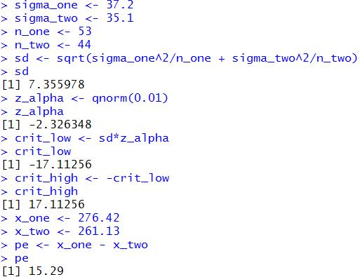
The R statements for those computations are:
sigma_one <- 37.2 sigma_two <- 35.1 n_one <- 53 n_two <- 44 sd <- sqrt(sigma_one^2/n_one + sigma_two^2/n_two) sd z_alpha <- qnorm(0.01) z_alpha crit_low <- sd*z_alpha crit_low crit_high <- -crit_low crit_high x_one <- 276.42 x_two <- 261.13 pe <- x_one - x_two pe
The console view of those statements is given in Figure 10.

Figure 10

The attained significance approach:

With the given values of the population standard deviations and the known sample sizes we compute the standard error as before, namely, 7.356. Then we take our samples and find the sample means, 276.42 and 261.13. We note that the difference 276.42 - 261.13 will be positive. Therefore, we need to find the probability of getting that value or higher from our distribution which has mean 0 and standard deviation 7.356. We can do this with a pnorm() function call. The result then needs to be multiplied by 2 because we are looking at a two-tailed test. We are answering the question "What is the probability of being that far away from the mean, in either direction?" We calculated one side so we need to double it to get the total probability. The one-side value is 0.0188, so the total will be 0.0376, a value that is larger than our level of significance, 0.02, in the problem statement. Therefore, we do not reject H₀ at the 0.02 level of significance.

The following R statements do these computations:
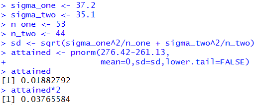
sigma_one <- 37.2 sigma_two <- 35.1 n_one <- 53 n_two <- 44 sd <- sqrt(sigma_one^2/n_one + sigma_two^2/n_two) attained <- pnorm(276.42-261.13, mean=0,sd=sd,lower.tail=FALSE) attained attained*2
The console image of those statements is given in Figure 11.

Figure 11

At this point is seems appropriate to try to capture these commands in a function so that we can use the function to solve any problem like these. Consider the following function definition:
hypoth_2test_known <- function( sigma_one, n_one, mean_one, sigma_two, n_two, mean_two, H1_type=0, sig_level=0.05) { # perform a hypothesis test for the difference of # two means when we know the standard deviations of # the two populations and the alternative hypothesis is # != if H1_type==0 # < if H1_type < 0 # > if H1_type > 0 # Do the test at sig_level significance. diff_sd <- sqrt( sigma_one^2/n_one + sigma_two^2/n_two ) if( H1_type==0) { z <- abs( qnorm(sig_level/2))} else { z <- abs( qnorm(sig_level))} to_be_extreme <- z*diff_sd decision <- "Reject" diff <- mean_one - mean_two if( H1_type < 0 ) { crit_low <- - to_be_extreme crit_high = "n.a." if( diff > crit_low) { decision <- "do not reject"} attained <- pnorm( diff, mean=0, sd=diff_sd) alt <- "mu_1 < mu_2" } else if ( H1_type == 0) { crit_low <- - to_be_extreme crit_high <- to_be_extreme if( (crit_low < diff) & (diff < crit_high) ) { decision <- "do not reject"} if( diff < 0 ) { attained <- 2*pnorm(diff, mean=0, sd=diff_sd)} else { attained <- 2*pnorm(diff, mean=0, sd=diff_sd, lower.tail=FALSE) } alt <- "mu_1 != mu_2" } else { crit_low <- "n.a." crit_high <- to_be_extreme if( diff < crit_high) { decision <- "do not reject"} attained <- pnorm(diff, mean=0, sd=diff_sd, lower.tail=FALSE) alt <- "mu_1 > mu_2" } result <- c( alt, sigma_one, n_one, mean_one, sigma_two, n_two, mean_two, diff_sd, diff, sig_level, z, crit_low, crit_high, attained, decision) names(result) <- c("H1:", "sigma_one", "n_one","mean_one", "sigma_two", "n_two","mean_two", "std. err.", "difference", "sig level", "z", "critical low", "critical high", "attained", "decision") return( result) }
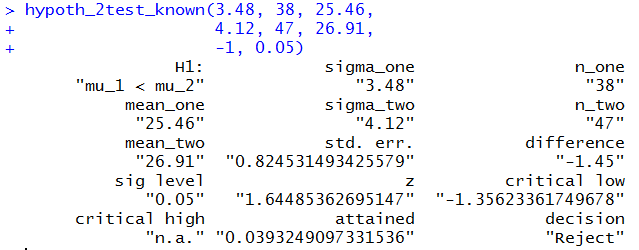
Once this function has been installed we can accomplish the analysis of Case: 8 above via the command
hypoth_2test_known(3.48, 38, 25.46, 4.12, 47, 26.91, -1, 0.05)
Figure 12 shows the console view of that command.

Figure 12

In a similar fashion, Case: 9 could have been handled via hypoth_2test_known(37.2, 53, 276.42, 35.1, 44, 261.13, 0, 0.02)
Figure 13 shows the console view of that command.

Figure 13

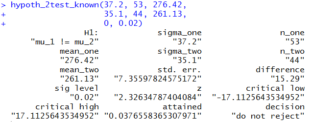
Clearly, the command shortens our work and still provides us with all of the details.

Case 10: We can use the function in a new problem. We start with two populations with known standard deviations, namely, 15.97 and 21.62. Furthermore, we know that the two populations have a normal distribution. As such we can "get away with" having slightly smaller samples. Our null hypothesis is that the means of the two populations is the same. Thus, we have H₀: μ₁ - μ₂ = 0 and our alternative hypothesis is H₁: μ₁ - μ₂ > 0. We want to test H₀ at the 0.025 level of significance. (This is a one-tail test.) We agree to take samples from each population, where the sample size is 24 and 28, respectively. Table 5 has the sample from the first population.

Table 6 has the sample from the second population.

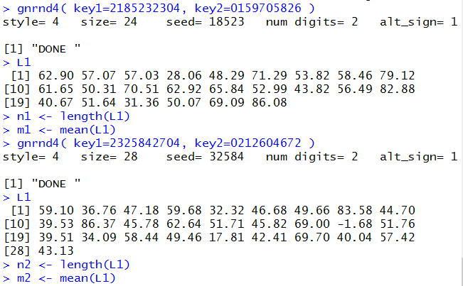
For this information we need to do a little processing. We want the sample size and the sample mean for each of the two samples. We can generate the data and get those values with the R commands:
gnrnd4( key1=2185232304, key2=0159705826 ) L1 n1 <- length(L1) m1 <- mean(L1) gnrnd4( key1=2325842704, key2=0212604672 ) L1 n2 <- length(L1) m2 <- mean(L1)
It was not necessary to display the data but it is nice to have the display so that we can confirm that we have correctly entered the gnrnd4() commands. The console view follows in Figure 14.
Figure 14

Then,to do the problem we just need the command
hypoth_2test_known(15.97, n1, m1, 21.62, n2, m2, 1, 0.025)
That command produces the output of Figure 15.
Figure 15

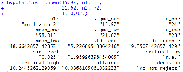
Figure 15 gives us the standard error, 5.227, the two sample means, 58.015 and 48.664, the difference of the means, 9.351, the critical value, 10.245 (there is only one since this is a one-tail test), the attained significance, 0.0368, and even the decision, do not reject. We would reach that decision using the critical value approach because the difference was not greater than the critical value, or by the attained significance approach because the attained significance was not less than the level of significance.

Table 7 presents some sample problems. The solution to those problems is given, case by case, in table 8. Please recall that the problems given above change every time that the page is reloaded. Because that is the case, we cannot provide a RStudio solution to the problems just given There is, however, a page that takes problems from a previously generated version of this page and displays both the tables, one giving the problems and the other giving the answers, and the RStudio solutions to those problems. That page of demonstrations is at Test for Comparing Means of Two Populations, Sigmas Known.

Return to Topics page
©Roger M. Palay Saline, MI 48176 February, 2016

Two Samples: σ known

Confidence interval for the difference μ1 - μ2

Hypothesis Testing for the difference of two means

Confidence interval for the difference μ₁ - μ₂