Figure 01
|
Remembering that
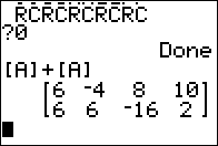
let us look at [A]+{A] as in Figure 01.
Itis pretty clear that the result is the same as if we just multiplied
every element of [A] by 2.
|
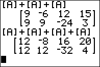
Figure 02
|
Figure 02 carries this forward by looking at
[A]+[A]+[A] and
[A]+[A]+[A]+[A].
The same pattern holds for these sums.
Back when we first learned about multiplying numbers, our
introduction was that multiplication represent repeated addition. That is, for numbers, (4)(3)
was just four 3's addedtogether, 3+3+3+3.
Now we will say the same thing as our way to introduce
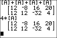
scalar multiplication of matrices. That is,4*[A]
reresents [A]+[A]+[A]+[A]. The 4 is a scalar, a numeric value.
We are multiplying that scalar times the matrix.
|
Figure 03
|
The calculator does this as shown in the bottom half of Figure 03.
The top half still holds the result of [A]+[A]+[A]+[A] and we can see that we get the
same answer either way.
|
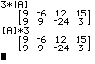
Figure 04
|
Figure 04 shows that we can, on the calculator, multiply the matrix by the scalar
on either the left or the right. (Of course, if 3*[A] is interpretted as adding three
[A]'s together, we have to understand that [A]*3 does not mean adding [A] 3's
together. Rather, we have a case of multiplying a scalar and a matrix and the
interpretation, in either case is repeating the matrix the number of times given
by the scalar.
In all of the cases shown, it is clear that the result of the scalar multiplication
is a matrix with each of the elements of the matrix being multiplied by that scalar.
|
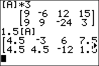
Figure 05
|
We continue that pattern when we look at 1.5[A]. First note that the TI-83/84 calculators
recognize implied multiplication so the
command 1.5[A] is understood to be 1.5*[A]. The result is
what we should expect, namely, it is a matrix with every value in it multiplied by 1.5.
|
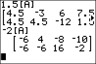
Figure 06
|
We can even multiply the matrix by a negative value, as in Figure 06.
The result follows the same pattern; multiply all the elements of the matrix by -2.
|
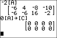
Figure 07
|
That pattern means that we if we have a matrix we can generate the zero
matrix for that given dimension by multiplying the known matrix by 0.
In Figure 07 we create a zero 2 x 3 matrix in [C] by multiplying
0 ime [A] and storing the result in [C].
|
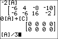
Figure 08
|
We often think of multipliation and division as being tied together.
In Figure 08, at the bottom,
we have a command that we might expect to be treated in a way similar
to scalar multiplication. Here we want to divide the matrix by 3.
But this does not work.
|
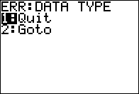
Figure 09
|
The effort resuts in an error. On the TI-83/84 calculators you cannot divide
a matrix by a scalar.
|
Figure 10
|
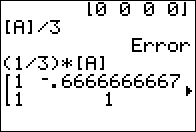
That does not mean that all is lost. Dividing by 3 is the same as multiplying by (1/3).
The command, shown in Figure 10, (1/3)*[A] is
a
scalar multiplication and it works just as expected.
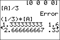
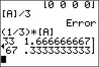
It does take us a while, Figures 10, 11, and 12 to see all of the result because
we need to scroll the calculator over the many digits of the various values.
Figure 10 shows the 1st and 2nd columns.
|
Figure 11
|
Figure 11 shows the 3rd column.
|
Figure 12
|
Figure 12 shows the 4th column.
.
|
Figure 13
|
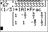
Modifying the same command by adding the  indicator
makes the output a little easier to read, as shown in Figure 13. indicator
makes the output a little easier to read, as shown in Figure 13.
|


 indicator
makes the output a little easier to read, as shown in Figure 13.
