Matrix: Multiply

Return to Roadmap 3

We can use the GNRNDM program with the key values -6723101206, 4443244234 and 0000000033 to generate the matrices: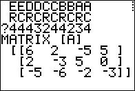

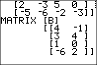
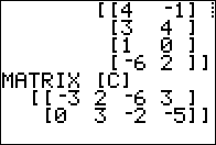
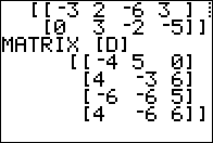
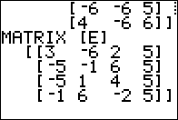
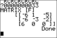
The calculator used to obtain the images below was a TI 84 Plus running the 2.55MP operating system and it was in the MATHPRINT display mode. These images merely reflect generating the matrices.

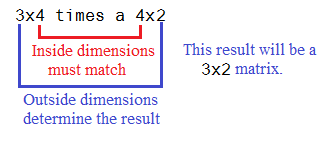
Our first example will be to multiply matrix [A] time [B]. We can do this because matrix [A] is a 3x4 matrix and [B] is a 4x2 matrix. We are allowed to multiply two matrices if the number of columns of the first is equal to the number of rows of the second. In this case we have 4 columns in [A] and 4 rows in [B]. The result of the multiplication will be a matrix that has dimensions equal to the number of rows of the the first matrix and the number of coulmns of the second matrix. In this case we have 3 rows in [A] and 2 columns in [B] so our result will be a 3 x 2 matrix. Or

Since we know that the result will be a 3 x 2 matrix, our problem becomes one of filling in the blank cells in:

To find the value in the 1st row, 1st column of the result we multiply the elements of the first row of the left matrix times the elements of the first column of the right matrix, and then add those products. In this case the sum of the products is ^–5.

To find the value in the 2nd row, 1st column of the result we multiply the elements of the second row of the left matrix times the elements of the first column of the right matrix, and then add those products. In this case the sum of the products is 4.

To find the value in the 3rd row, 1st column of the result we multiply the elements of the third row of the left matrix times the elements of the first column of the right matrix, and then add those products. In this case the sum of the products is ^–22.

To find the value in the 1st row, 2nd column of the result we multiply the elements of the first row of the left matrix times the elements of the second column of the right matrix, and then add those products. In this case the sum of the products is 12.

To find the value in the 2nd row, 2nd column of the result we multiply the elements of the second row of the left matrix times the elements of the second column of the right matrix, and then add those products. In this case the sum of the products is ^–14.

To find the value in the 3rd row, 2nd column of the result we multiply the elements of the third row of the left matrix times the elements of the second column of the right matrix, and then add those products. In this case the sum of the products is ^–25.

All of this should convince you that finding teh product of two matrices takes a lot of work. In this case there were 42 separate arithmetic operations to be performed to get our six values in the result. Clearly, the calculator should be able to help us in this.

Figure 01	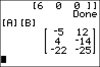Remember that the TI-83/84 calculators, for the most part, understand implied multiplication. Thus, forming the command [A][B} tells the calculator to compute the product of [A] and [B]. The result, identical to our hand prepared result above, is shown in Figure 01.
Figure 02	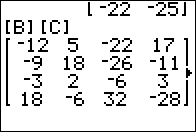[B][C] means multiplying a `4 x 2` times a `2 x 4` yielding a `4 x 4` product.
Figure 03	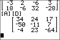[A][D] means multiplying a `3 x 4` times a `4 x 3` yielding a `3 x 3` product.
Figure 04	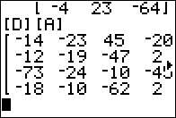[D][A] means multiplying a `4 x 3` times a `3 x 4` yielding a `4 x 4` product. This is clear evidence that matrix multiplication is not commutative! The result in Figure 03 is totally different from the result in Figure 04.
Figure 05	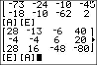Figure 05 shows [A][E], a perfectly valid operation, and then it shows the command [E][A]. This latter command should cause us problems because it is an attempt to multiply a `4 x 4` matrix times a `3 x 4` matrix, in which case the "inside" values do not match.
Figure 06	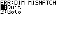Figure 06 show the calculator response noting that there is an error in that command.
Figure 07	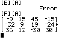Figure 07 shows that it is OK to multiply a `3 x 3` amtrix times a `3 x 4` matrix.
Figure 08	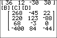Figure 08 is an attempt to look at, though not to prove that, matrix multiplication is associative. In this case we let the calculator do the operations in whatever order it wants, which will be left to right.
Figure 09	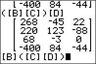Figure 09 forces the calculator to do the left multiplication first. THe result of that is then multiplied by the last matrix. We see that we get the same answer that we had in Figure 08. The, in Figure 09 we create the command that will force the calculator to do the right multiplication first with the first matrix, [B], to be multiplied by that result. If matrix multiplication is associative then this should work.
Figure 10	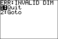Unfortunately, our command at the end of Figure 09 causes an error.
Figure 11	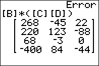The problem is a "fault" in the calculator. It does not like the parentheses the way we had tehm. In particulr, for some reason, the TI-83/84 calculators do not understand the implied multiplication of [B] with the parenthetical expression to its right. However, if we force the calculator to recognize the multiplication, as shown in Figure 11, then all works out as we would expect.
Figure 12	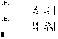As we saw, unlike numeric multiplication which is both commutative and associative, matrix multiplication is not commutativealthough it is associative. There is another difference between numeric and matrix multiplication. With numbers such as a and b we know that if we are told that *ab = 0 then it must be the case that either one or both of a or b must be 0. However, consider the two matrices shown in Figure 12. Neither is the zero** matrix. In Figure 13 we will multiply those two matrices.
Figure 13	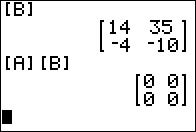The result of multiplying these two non-zero matrices is the zero matrix.