Matrix: Inverse

Figure 01	Figure 01, taken from the matrix editor, displays matrix [A]. We will use this in the process of finding its inverse matrix.
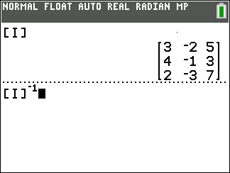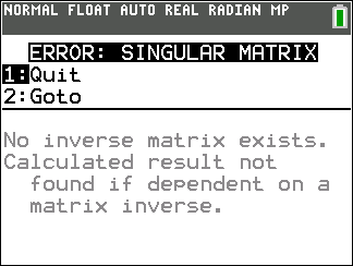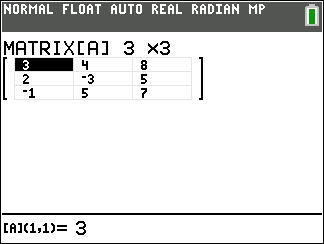
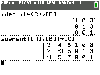
Figure 02	In Figure 02 we start by creating a 3 x 3 identity matrix and storing that in [B]. Then we go forward and paste the two matrices together to form a new 3 x 6 matrix which we store in [C].
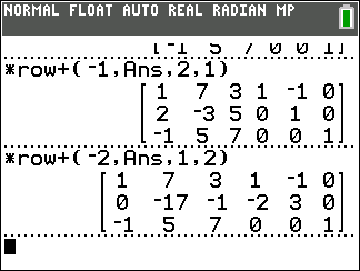
Figure 03	The process will be to use the elementary row operations to convert the left 3 columns of the matrix into the identity matrix. Once that is done then the right three columns of the matrix will hold the desired inverse of the original 3 x 3 matrix. Looking back at the lower half of Figure 02 we see that if we multiply row 2 by -1 and then add that to row 1 we will create a 1 in the first row, first column position. Our 3 x 6 matrix at the end of Figure 02 is not only stored in [C] but also stored in Ans. We will just work on the version stored in Ans. The command *row+(-1,Ans,2,1) does that operation, and it shows the resulting new value of Ans in the top halpf of Figure 03. Next we want to genreate 0's below that 1. The first one we do is take -2 times row 1 and add it to row two. That command is *row+(-2,Ans,1,2) and the lower half of Figure 03 gives us the result.
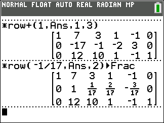
Figure 04	To change the -1 in row 3, column 1 in the current Ans we use *row(1,Ans, 1,3). With that command we have completed the taks of getting 0's below the 1 in row 1, column 1. Next we need to get a 1 in the second row, second column. Currently there is a -17 there. One way to make that value into a 1 is to multiply the row by -1/17. That is the gist of the next command shown in the middle of Figure 04, *row(-1/17,Ans,2). Notice that we have added the to the command so that the calculator displays the result as fractions where possible. The result shows that we were successful.
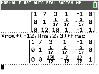
Figure 05	Next, to change the value (there is only one) below the diagonal in the second column to 0, we can add -12 times the second row to the third row. That command is *row+(12,Ans,2,3).
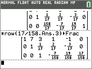
Figure 06	We now want to make the diagonal element in the third column be 1. Its current value, at the end of Figure 05, is 158/17. We can multiply that row by 17/158 via the command *row(17/158,Ans,3).
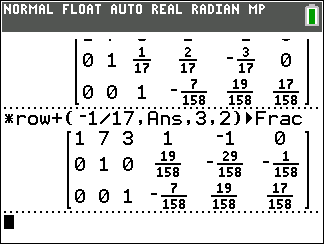
Figure 07	Now that we have the diagonal as 1's and the values below that diagonal as 0's we turn our attention to making the values above the diagonal be 0's ass well. We start with the third column and work back toward the first. Back in Figure 06 we see that we have 1/17 in the second row third column. We can make that a 0 with the command *row+(-1/17,Ans,3,2).
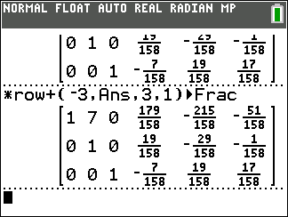
Figure 08	To change the 3 in the first row third column we use the command *row+(-3,Ans,3,1). That will complete our work in the third column. After that we move back to the second column.
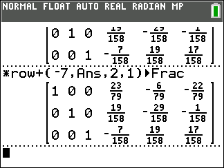
Figure 09	To change the 7 in the first row second column we use the command *row+(-7,Ans,2,1). Once that is done we have finished our work. We have the identity matrix in the first three columns. The last three columns hold the inverse of the original matrix. In the "old days" when we had to do this all by hand we would just copy those final three columns as our 3 x 3 inverse matrix. There is no "nice" single command to pull out those columns on the calculator although after we see the short way of getting the inverse, in Figure 10, we will look at some ways to do this without copying each of the values.
Figure 10	What we have seen in the ffigures above is the long, step by step, method of finding the inverese by using the elementary row operations. The process is merely an algorithm, a set of commands that we can follow, that takes us from an initial condition (the original matrix) to the final condition (the inverse matrix in the final columns). We could write a program to do this. 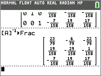In fact, the makers off the TI-83/84 have done that with the added benefit of pulling out the answer as a new 3 x 3 matrix. 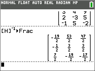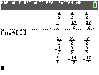To get the TI-83/84 calculators to perform that program you just need to give the name of the original matrix folowed by the "reciprocal sign", the -1 that is displayed when we press the key. That is the command, followed by the command, that you see in Figure 10. That one command produces the desired result.
Figure 11	Figure 11 merely shows us the matrix [C] that we construced earlier.
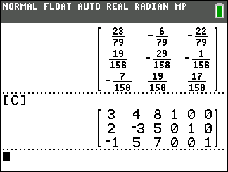
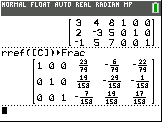
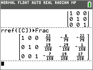
Figure 12	Once we have [C], rather than go through the long set or elementary row operations, we could have just asked the calculator to do the rref( process on the matrix. [Recall that such a process is the "reduced row-eschelon form.] In Figure 12 we see that using the rref( function had us go from what we had back in Figure 02 to the solution that we found in Figure 09. Of course, we still have the answer as part of a 3 x 6 matrix here.
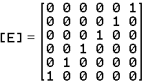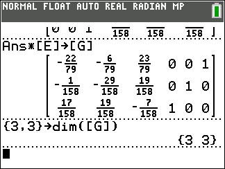
Figure 13	In order to understand Figure 13 we need to know that we have previously defined [E] as . That 6 x 6 matrix, as ou see, is all o's except for the values in the "backwards" diagonal, which are all set to 1. Figure 13 shows the result of multiplying the answer, Ans, of Figure 12 by [E] (on the right). what you see is that the result is just the old answer of Figure 12 but flipped left to right. By oing this we have placed the "flipped" version of the nverse matrix into the first three columns of our 3 x 6 matrix.
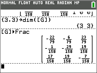
Figure 14	Now we take advantage of the fact that the TI-83/84 calculators allow us to change the dimensions of a matrix and to retain any values that have not been cut off. The command {3,3}→dim([G]) will change [G] to a 3 x 3 matrix, retaining the first three columns. The subsequent command just displays our new [G]. It contains the flipped version of the inverse matrix. All we need to do is to flip it back.
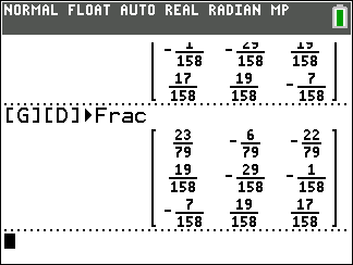
Figure 15	Figure 15 intrduces yet another matrix that we defined previously, namely . We just have to multiply [G] by [D], on the right, to flip it again left to right. The result is exactly the inverse matrix that we want.
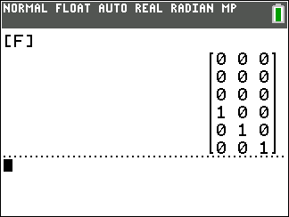
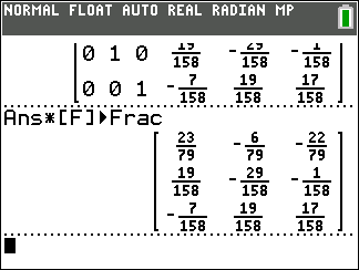
Figure 15.1	Assuming that the funny matrix operations that we have seen in Figure 12 through Figure 15 have been of some interest, we will go one step further. Figure 15.1 introduces a new matrix, [F], that is a somewhat strange 6 x 3 matrix. Now the top half of the matrix is all 0 values and the bottom is looks like the identity matrix.
Figure 15.2	Figure 15.2 merely recreates our 3 x 6 matrix answer.
Figure 15.3	Then, in Figure 15.3, we just muliply that answer by [F], on the right, and our solution inverse matrix appears, in one step, as a 3 x 3 matrix.
Figure 16	Before we leave the topic, let us look at a different example. Figure 16 shows a new matrix, [H].
Figure 17	In Figure 17 we create and display the inverse matrix for [H].
Figure 18	In Figure 18 we simply store that inverese matrix in [I].
Figure 19	And in Figure 19 we ultiply our original matrix, [H] by its inverse, [I], and we do it twice, once on the left and once on the right. The result is that the product is the identity matrix.
Figure 20	Finally, for Figure 20 we have put a different matrix into [I] and then we have formed the command to find the inverse of that matrix.
Figure 21	The surprising result is an error message. It turns out that the perfectly good looking matrix that we had in [I] does not have an inverse. You may recall that with numbers, the only number that does not have an inverse is 0, the addative identity value. Certainly, any square zero matrix will not have a multiplicative inverse. However, what we have seen in Figure 21 is that even some non-zero matrices do not have multiplicatiove inverse.