and
and  into a
TI-83/84 calculator.
Note that the calculator display is slightly different
depending on the display setting of the calculator.
There are two values for that setting MATHPRINT
and CLASSIC. The TI-83 and TI-83 Plus calculators
only have the CLASSIC mode, as do the earlier versions of the TI-84 Plus
calculators.
Newer versions of the TI-84 Plus calculator, along with older ones that have had their
operating system upgraded to version 2.53 or higher, have both settings.
The calculator used to obtain the images below was a TI 84 Plus running the 2.55MP
operating system.
into a
TI-83/84 calculator.
Note that the calculator display is slightly different
depending on the display setting of the calculator.
There are two values for that setting MATHPRINT
and CLASSIC. The TI-83 and TI-83 Plus calculators
only have the CLASSIC mode, as do the earlier versions of the TI-84 Plus
calculators.
Newer versions of the TI-84 Plus calculator, along with older ones that have had their
operating system upgraded to version 2.53 or higher, have both settings.
The calculator used to obtain the images below was a TI 84 Plus running the 2.55MP
operating system.
 key to get the sidplay in Figure 01.
[Note that if you are using a TI-83 or TI-83 Plus or a TI-84 Plus that does not have
the next at the bottom of the screen then
you can just skip to Figure 03 because you have no choice but to be in CLASSIc
display mode.
key to get the sidplay in Figure 01.
[Note that if you are using a TI-83 or TI-83 Plus or a TI-84 Plus that does not have
the next at the bottom of the screen then
you can just skip to Figure 03 because you have no choice but to be in CLASSIc
display mode.
Use the
 repetedly to move to the next at
the bottom of the screen. This will produce the image in Figure 02.
repetedly to move to the next at
the bottom of the screen. This will produce the image in Figure 02.
 . If the black highlight
had been on the MATHPRINT option, as in
. If the black highlight
had been on the MATHPRINT option, as in
 then we would have moved the blinking cursor
to the right, using the
then we would have moved the blinking cursor
to the right, using the  key to change
the blinking item to cover the CLASSIC option, and then we would have pressed
the
key to change
the blinking item to cover the CLASSIC option, and then we would have pressed
the  key to make that the selected option.
That is the status shown in the display
in Figure 02.
key to make that the selected option.
That is the status shown in the display
in Figure 02.
Leave Figure 02 by the sequence
 .
.


 .
That creates the image shown in Figure 03.
.
That creates the image shown in Figure 03.
 to have the calculator perform the command.
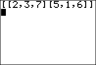
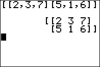
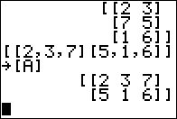
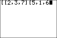
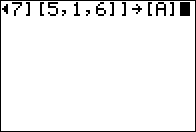
The result is shown in Figure 04. Note how that result mimics the characters
that we used to input the matrix. We can see the two rows and 3 columns, and the
values in the matrix are aligned. The commas have disappeared.
to have the calculator perform the command.
The result is shown in Figure 04. Note how that result mimics the characters
that we used to input the matrix. We can see the two rows and 3 columns, and the
values in the matrix are aligned. The commas have disappeared.
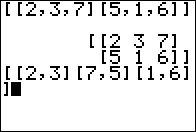 to have
the calculator process the command and produce Figure 06.
to have
the calculator process the command and produce Figure 06.
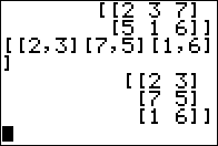
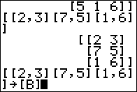
It is important to note that we have created these matrices but they have not been "stored" in a variable. In fact, having created the second one, shown in Figure 06, we have lost the first. We need to save these matrices in the variables that the calculator provides to hold such entities.
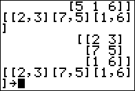
 key, the symbol to store the new value.
However, now we must find the specific variable [B].
As tempting as it might be, we cannot just type those
characters. Instead we need to open the MATRIX menu
via the keystrokes
key, the symbol to store the new value.
However, now we must find the specific variable [B].
As tempting as it might be, we cannot just type those
characters. Instead we need to open the MATRIX menu
via the keystrokes  .
This show take us to Figure 08. [Note:it is rare to find someone using a
a TI-83 (not the 83 Plus) anymore. But if you have an old TI-83 then the
keys are sightly different. On that calculator you open the matrix menu shown in
Figure 08 via the single
.
This show take us to Figure 08. [Note:it is rare to find someone using a
a TI-83 (not the 83 Plus) anymore. But if you have an old TI-83 then the
keys are sightly different. On that calculator you open the matrix menu shown in
Figure 08 via the single  key.]
key.]
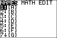 to move the highlight to the second item as shown in Figure 09.
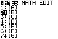 to actually choose that item. [In fact, we could use the alternative of just
pressing the "2" key, and we could have done that without having the item selected.]
to actually choose that item. [In fact, we could use the alternative of just
pressing the "2" key, and we could have done that without having the item selected.]
 to have the calculator process the
command.
to have the calculator process the
command.
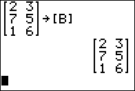
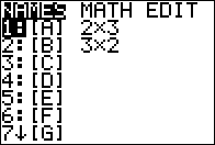 ,
we can see the fruits of our labor.
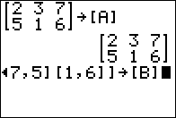
The screen shows tha the two matrices [A] and [B] have been
assigned values and that the former is a 2 x 3 matrix while the
latter is a 3 x 2 matrix.
,
we can see the fruits of our labor.
The screen shows tha the two matrices [A] and [B] have been
assigned values and that the former is a 2 x 3 matrix while the
latter is a 3 x 2 matrix.
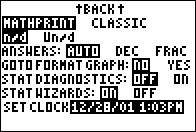 key to return to the MODE menu and then
repeatedly use the to move to that menu's second page.
There we change the display option to MATHPRINT, as in the
portion shown in Figure 13.
key to return to the MODE menu and then
repeatedly use the to move to that menu's second page.
There we change the display option to MATHPRINT, as in the
portion shown in Figure 13.
 key to move to Figure 17.
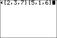
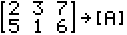 .
The second is that the matrix now looks more line a matrix
with just the single set of large square brackets
enclosing the rectangualr array of values, as in
.
The second is that the matrix now looks more line a matrix
with just the single set of large square brackets
enclosing the rectangualr array of values, as in
 .
. Also in Figure 17 we have entered the command to create and store the second matrix. Once there we can press the
key to havve the
calculator perform that command. The result is shown in Figure 18.
by