Matrix: Addition (GNRNDM)

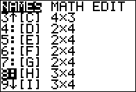
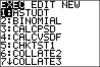
Figure 01	Open the PROGRAM menu by pressing the key.
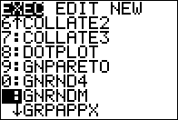
Figure 02	Use the key to find and highlight the GNRNDM program. Then press the key to move to Figure 03.
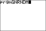
Figure 03	Figure 03 shows the command needed to actually run the progrm. We just need to press to have the calculator run the GNRNDM program
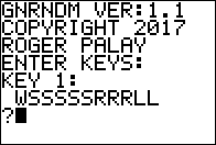
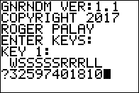
Figure 04	The program starts with a request for the value of the first key. The program tries to convey the meaning of the key value: we have one Wasted digit or symbol (explained later), 5 Seed value digits for the random number generator, 3 Range digits, and 2 Start digits. The program uses these to determine the lowest allowd value in the matrix (SS) and the range of values allowed (RRR).Thus, the highest value in the matrices will be LL+RRR. The Wasted value is ignored, unless it is a negative sign, in which case the LL value is taken to be negative.
Figure 05	We respond, in Figure 05, with the value 322597401810, which means that the lowest value in the generated matrices is 10 and the highest is 28. You might check the ten matrices shown above to verify that those limits were in fact used. Press to move forward.
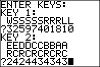
Figure 06	The program prompts for the second key. This time the program tries to help us by giving us the hint EEDDCCBBAA RCRCRCRCRC to tell us that the two leftmost of the ten digits will specify the number of rows and columns in matrix E, the next two digits will specify the number of rows and columns in matrix D, and so on. The response that we enter, 2424434343, specifies that E is a 2x4, D is a 2x4, C is a 4x3, B is a 4x3, and A is a 4x3. Press to give those values to the program.
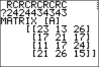
Figure 07	The program starts to do its work. It creates and displays matrix A and waits for us to press to move on.
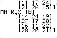
Figure 08	It creates and displays matrix B and waits for us to press to move on.
Figure 09	It creates and displays matrix C and waits for us to press to move on.
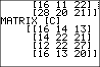
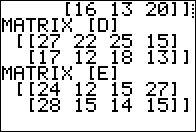
Figure 10	It creates and displays matrix D and waits for us to press to move on. Then it creates and displays matrix E and waits for us to press to move on.
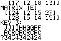
Figure 11	Now the program asks for the row and column sizes of the last five matrices, J, I, H, G, and F. Our response of 3434342424 specifies that J is a 3x4, I is a 3x4, H is a 3x4, G is a 2x4, and F is a 2x4. Press to give those values to the program.
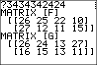
Figure 12	It creates and displays matrix F and waits for us to press to move on. Then it creates and displays matrix G and waits for us to press to move on. .
Figure 13	It creates and displays matrix H and waits for us to press to move on.
Figure 14	It creates and displays matrix I and waits for us to press to move on.
Figure 15	It creates and displays matrix J and the program is done.
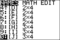
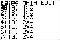
Figure 16	We use the sequence to open the MATRIX menu shown in Figure 16. This provides a quick confirmation on the size of the matrices now in the calculator.
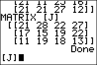
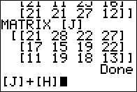
Figure 17	To get to Figure 17; we use the key to move the highlight down to show the remaining matrices. We press to paste the name of the highlighted matrix, in this case [J], onto the main screen as is shown in Figure 18.
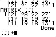
Figure 18	To do matrix addition we just need to form the command using the + sign. We can accomplish this via the key, giving the result shown in Figure 19.
Figure 19	In this example we want to add [J] to [H} so we need to get the name [H]to end our command. We cannot type that name. Rather, we need to return to the matrix menu, via and then use the key to move the highlight to the desired matrix name. This situation is shown in Figure 20.
Figure 20	Press to paste [H] onto the home screen, shown in Figure 21.
Figure 21	With the command completed we just need to press to have the calculator perform that command.
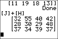
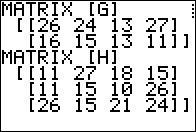
Figure 22	The result is shown in Figure 22. Here we see that It should be clear that the algorith used to add two matrices is to form a new matrix, of the same dimension, where the elements of the new matrix are just the sum of the corresponding elements of the original two matrices. In this example, the 32 in the first row, first column of the answer is just the sum of the 21 and 11 that are in the same position in [J] and [H], respectively. The requirement for adding two matrices is that they have to have the same dimensions, i.e., they must have an identical number of rows and an identical number of columns. Our example worked because the two original matrices each had 3 rows and 4 columns.
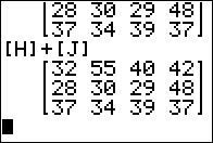
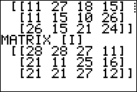
Figure 23	One important property of addition that we learned when dealing with numeric values is that the opertion of addition for numbers is commutative, which means that x + y = y + x. Considering that to add two matrices we just add the respective component elements of the matrices we should expect that the operation of addition for matrices is commutative. Giving an example does not prove that this is true, but Figure 23 does show that [H]+[J] gives the same result as we had for [J]+[H].
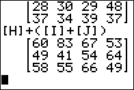
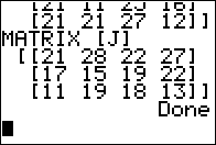
Figure 24	Another numeric property of addition is that the operation is associative. That means that for any numbers, x, y, and z it is always true that x + (y + ) = (x + y) + z. We can give an example of this for matrices. In Figure 24 we find [H]+([I]+[J]).
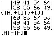
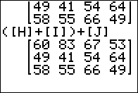
Figure 25	Then in Figure 25 we find ([H]+([I])+[J]. The result is the same. Again, this is not a shock given that when we add matrices we are just adding corresponding elements from the matrices involved. This is not a proof. Rather it is an illustration the addition of matrices is associative.
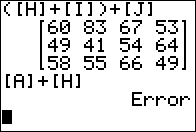
Figure 26	What happens on the calculator if we try to add matrices that do not have the same dimensions? We can try this via [A]+[H], trying to add a 4x3 and a 3x4 matrices. Figure 26 shows the command. Press to ask the calculator to perform the command.
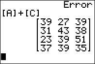
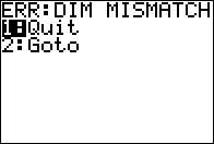
Figure 27	The calculator detects the error and reports it as shown in Figure 27. We can press Press to choose to Quit the task. This returns us to the main screen, shown in Figure 28.
Figure 28	Note that the alculator marked the previous command as an Error.
Figure 29	We saw that we could not add [A] and [H], but we can add [A] and [C]. The result is shown in Figure 29.