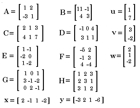

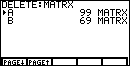
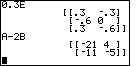
 to display a screen similar to this.
| All of the options on the left,
and only the options on the left, should be highlighted. If your screen does
not appear like this, then you should fix it. Use the cursor control keys to move up and down,
left and right on the screen. Then use the  key to select the
desired option.
To get out of the review of modes, press the key to select the
desired option.
To get out of the review of modes, press the  . . |

|
Next we want to remove any confusion about the names of matrices already stored
on the calculator. This is not an essential step, but it does
show you how to remove existing matrices from the calculator. To do this we
will press the  keys. This will
open a menu, as seen in the Figure 3. keys. This will
open a menu, as seen in the Figure 3.
|
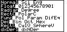
| Now that we have the MEM menu available, we have some options.
The first option, RAM, displays the random access memory report. We
do not need to do this now. The second option, DELET, will allow us to
delete any of the variables previously stored in the calculator. That is the
option we want, so press  to select DELET. to select DELET.
|

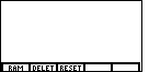
| Once DELET has been chosen, the word DELETE is displayed, and the menu
items change, as shown in Figure 4. The new options are really asking what "class"
of variable to we want displayed so that we can select the items to delete. Choosing the
first option, ALL, would cause all of the variables to be displayed. Choosing the fourth
option, LIST, would cause only the LISTs to be displayed. We want to delete old matrix
variables. MATRIX is not an option on this menu. However, press the
key to cause the calculator to scroll over to new
options for the menu, as seen in Figure 5.
|
|
Here the menu has changed so that MATRX is now option 1. We want
do delete a matrix or two, so we need to press  to
select the MATRX menu option. to
select the MATRX menu option.
|
|
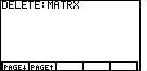
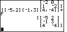
As a result of selecting the MATRX menu option, the calculator displays a
screen that starts with DELETE:MATRIX and then lists each of the matrices
that have been defined on the calculator. Naturally, your screen, at this point,
may well be different. You will see a list of the defined matrices
on your calculator. On my
calculator there were two, A and B, as shown in Figure 6.
The numbers to the right of the screen give
the size, in bytes, of each matrix.
At this point, in Figure 6, the matrix A is selected.
To actually delete the selected matrix, press the
|
| Now that we have deleted the desired matrices, we need to
get out of the DELETE process. Do this by pressing the
key. This will return the calculator to a blank screen (as in Figure 2). Now we can
begin to enter the various matrices defined in problem 5 on page 135 of the text.
First we will enter the matrix A.
|
| We could use the Matrix menu and enter the matrix as demonstrated earlier in
the course. However, at this point we will just enter the matrix directly. To do this we enter
the [ character as
 to open the matrix.
Then, we enter each row of the matrix enclosed between
[ and ], with the numbers separated by commas.
Therefore, we continue with the first row as to open the matrix.
Then, we enter each row of the matrix enclosed between
[ and ], with the numbers separated by commas.
Therefore, we continue with the first row as
 
  and the second row as
 and then we end the matrix with a closing ] by pressing
.
and then we end the matrix with a closing ] by pressing
.
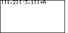
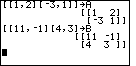
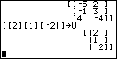
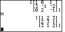
That sequence, [[1,2][-3,1]] is the matrix, but we want to store the matrix in a
variable called A.
To do this, press |
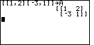
| Press the key to
accept the line typed in Figure 8. This will produce Figure 9. Not only is the
matrix stored into a variable called A, but it is displayed as the answer.
Note that the TI-85 is case-sensitive. That is, the names A and a represent different
variables. Therefore, on the TI-85 we must be careful to type the proper case for any variable.
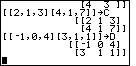
We can move ahead by typing the matrix for B
and then storing that matrix in B.
|
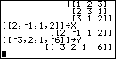
| Figure 10, which builds on Figure 9, is the result of the key strokes
to open the matrix,
then the first row
,
the second row as
 ,
then the end of the matrix by pressing
,
assigning the matrix to B by pressing
,
then the end of the matrix by pressing
,
assigning the matrix to B by pressing
  ,
and finally to accept and perform the command.
Note that the entry and display of A are still visible at the top of the screen. ,
and finally to accept and perform the command.
Note that the entry and display of A are still visible at the top of the screen.
|
| Most of the remaining matrices are entered the same way. As new matrices are entered, the display scrolls off the top of the screen. Thus, Figure 11 shows the subsequent entry of both C and D, but the [4, 3 ]] at the top is left over from the end of the display of the B matrix. Note that for these matrices, C and D, there are three numbers in each row. |
|
Although the calculator may allow some less formal way of entering U and V,
Figure 12 follows the strict pattern established above
for A, B, C, and D. That is,
we start each matrix with [, we enter
each row as [ followed by a set of
numbers separated by commas and ending with ],
and we end the matrix with ]. For matrix U there is
only one number per row. The same is true for matrix V. Note that in these examples, we are using upper case letters for the matrices U, V, W, X, and Y. We could have used lower case letters but this would require many more keystrokes. |
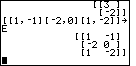
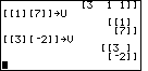
| Figure 13 shows the entry for matrix E, which has three rows, but only two elements (numbers) in each row. |
| Figure 14 shows the entry for matrix F, which also has three rows, but only two elements in each row. |
| Figure 15 displays the entry of matrix W. This follows the pattern for both matrix U and matrix V in that there is only one element per row. However, for matrix W there are three rows. |
| Figure 16 displays the entry of matrix G, the largest matrix so far with three rows and three columns. |
| If you have been following along on the calculator, or just observing
the keystrokes needed to generate a matrix, it must be clear that it takes
many keystrokes to generate even one of the screens displayed here.
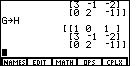
We could generate matrix H in the same manner used for the earlier matrices.
However, starting with Figure 17, we will look at an alternative method that illustrates
some other features of the calculator.
The middle of Figure 17shows the command to take the matrix stored in G
and copy it to H. The keystrokes are
|
| Figure 18 represents the result of the keystrokes
 , to open the MATRIX menu.
We want to edit matrix H so that we can change the elements of that matrix from
their current value (as copies of G) to the desired values. To do this, press
to select the EDIT menu item. , to open the MATRIX menu.
We want to edit matrix H so that we can change the elements of that matrix from
their current value (as copies of G) to the desired values. To do this, press
to select the EDIT menu item.
|
| The calculator responds by asking for the name of the matrix to edit, and displaying
the already defined matrix names at the bottom. The first set of matrix names was
A B C D E.
To get to the set of names displayed at the bottom of Figure 19, press the
button.
|
|
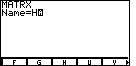
Now it is easy to fill in the alswer to the question of which matrix to enter.
We press  to select H. This produces Figure 20.
To move to Figure 21, press the . to select H. This produces Figure 20.
To move to Figure 21, press the .
|
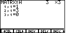
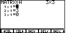
| When you you press the ENTER to leave Figure 20, the
calculator brings up Figure 21, and it highlights the initial
3 at the top of the screen. The "3 X 3"
allow you to change the size of the matrix. The initial value represents the number
of rows. The second value represents the number of columns. We do not want
to change the size of this matrix, so we leave the 3
as is by pressing .
|

|
Having accepted the number of rows, the calculator
moves to Figure 22
to allow a change in the number of columns. The second 3
at the top of the page is now highlighted. We do not want to change this
values so press to accept it.
|
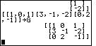
For this demonstration we will use a different approach. This approach
concentrates on using the ENTER key, it ignores the cursor keys, and it
uses a systematic approach to moving through the ROWS of the matrix.
We start at the
top left element and move across each column before moving to the next row.
|
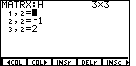
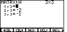
In Figure 23, the element at row 1 column 1 is highlighted.
Remember that the current values are a copy
of matrix G.
We want to change the values to hold matrix H,
which also starts with a 1. Therefore, we press
to select the current value, 1,
as the new value for element 1,1.
|
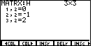
| In Figure 24, the calculator has moved to the first row of the second column. In the sceen capture of Figure 24, the cursor block is covering the proposed value of 0. On the real screen that block is blinking. Figure 24a shows the screen without the cursor block. |
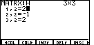
| Now, we want to change the value in row 1 column 2 to be a 2. Figures
24 and 24a show the blinking cursor at the current value of 0. Press
to specify the new value. The 2 is displayed,
and the cursor moves to the right as seen in Figure 24b.
|
|
In Figure 24b, the cursor is at a position so that more of the number to go into row 1
column 2 can be specified.
There is no more to the number, so
press again to accept the value.
|
|
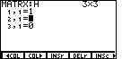
Having accepted the value of element 1,2 the calculator moves to the next element,
the one at row 1 column 3. This is the condition shown in Figure 25.
We want to change this
element to the value 3.
To do this, just press the keys for the new value, in this case, press
.
|
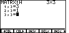
|
Because we entered a value in position 1,3 at the end of Figure 25, the calculator
moves to the next element, in this case the element at row 2, column 1.
The blinking cursor is shown in Figure 26 as covering up the original 3.
We want to change the value to a 2.
Press .
|
|
| This produces Figure 27.
Then,
press to accept that value, and move on to
the next element.
This process is to be repeated for the rest of the matrix. Because we are using the EDIT screen to change the values in H, we need only use the numeric keys and the ENTER key. This avoids the repeated use of the "2nd" key, the left and right braces, and the comma key. |
|
When you are done modifying the matrix, at the 3,3 element, the last ENTER key leaves the
focus at that same 3,3 element, as in Figure 28. To get out of the EDIT mode, use the
key.
|
| Having left the EDIT screen, we are returned to the mainscreen, as shown in Figure 29. |
|
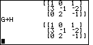
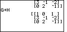
To see the changes that we made in the matrix, just type the name of the matrix
 and press
. Figure 30 shows this and the resulting display of the
H matrix. and press
. Figure 30 shows this and the resulting display of the
H matrix.
|
| Now we will finish our data entry the old way in Figure 31, directly entering the matrix for X and Y. Note that each matrix has one row. There is a slightly shorter way to enter a one-row matrix, calling it a VECTOR. However, for our purposes, we will stay with the idea of starting the matrix with [, then starting and stopping each row with [ and ], and then ending the matrix with ]. |
|
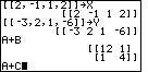
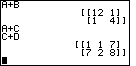
Now we are ready to do the problems that are in the book. To do
problem 7 press 
 and
to generate A+B.
Then press to perform the addition.
The sum of the two matrices is displayed.
This is shown in the middle of Figure 32.
Going back to the original values of A and B
it is easy to see how A+B is formed.
The new matrix looks like the original ones,
but each element of the answer is the sum of the
corresponding elements of the original matrices. and
to generate A+B.
Then press to perform the addition.
The sum of the two matrices is displayed.
This is shown in the middle of Figure 32.
Going back to the original values of A and B
it is easy to see how A+B is formed.
The new matrix looks like the original ones,
but each element of the answer is the sum of the
corresponding elements of the original matrices.
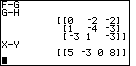
We finish Figure 32 by stating the addition of problem 8.
We do this by pressing |
|
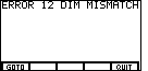
Figure 33 displays an error message at the top and a menu at the bottom. The error
is the result of our command A+C.
We can not add matrices unless they have the same number of rows and columns.
Matrix A is a 2x2 matrix (2 rows and 2 columns), but
matrix C is a 2x3 matrix [2 rows and 3 columns]. Therefore, addition of A and C is
not defined, and our attempt to add the two matrices causes the error.
We can press  to select option 5, QUIT, from the menu. to select option 5, QUIT, from the menu.
|
|
C and D are the same size. We say that each is of "order 2x3".
Thus we should be able to add them, as required in problem 9.
Figure 34 shows the result of

 .
Again, the sum has the same "order" as did the two original matrices, 2x3, and each
element of the answer is the sum of the corresponding elements of the original matrices. .
Again, the sum has the same "order" as did the two original matrices, 2x3, and each
element of the answer is the sum of the corresponding elements of the original matrices.
|
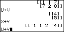
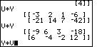
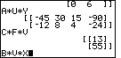
| Figure 35 shows results of problems 10 and 11, and the start of problem 12. The first two work, and give results that we should have been able to predict. The final problem, U+Y, has been stated, but it is waiting for the ENTER key to be pressed before it is executed. |
|
|
Pressing the at the end of Figure 35 casues an error, as seen in
Figure 36. The error is caused by U and Y having different "orders".
The "order" of U
is 2x1 and the "order" of Y is 1x4. Therefore, addition of these two matrices is not defined.
Press to QUIT the problem.
|
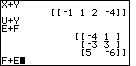
| Figure 37 shows the remains of Figure 36, problem 13 (E+F), and the statement of problem 14 (F+E). We should note the answer to problem 13, and verify that the addition is working as expected. |
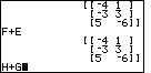
| Figure 38 shows the result of problem 14 (F+E) and the statement of problem 15. It is important to note that problems 13 and 14 demonstrate the fact that matrix addition is COMMUTATIVE. That is, there is no difference between E+F and F+E. The answer to problem 13 is seen at the top of the screen, while the answer to problem 14 is seen at the bottom. The answers are identical. |
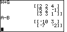
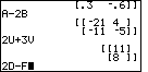
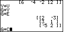
| The previous screen had the statement of problem 15. Figure 39 shows the result of doing H+G and the result of problem 16, A-B. We can verify that subtraction of matrices is similar to addition of matrices. The answer is the same "order" as the original matrices, and each element of the answer is the difference of corresponding elements of the original matrices. |
|
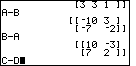
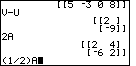
Since subtraction of numbers is NOT commutative, we would not expect
the subtraction of matrices to be any different. Figure 40 verifies this.
It shows the results of both A-B and B-A.
The two answers are opposites of each other, just as 7-4 and 4-7 generate opposite
answers. Figure 40 concludes with a statement of problem 18. |
| Figure 41 gives the results of both problem 18 and problem 19. |
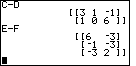
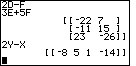
| Figure 42 starts with the answer to problem 19, E-F, and then continues with problem 20, F-E, and its answer. Again, we see that matrices of the same "order", in this case 3x2, can be subtracted, but that the order of the matrices does make a difference in the result. Figure 43 concludes with a statement of problem 21. |
|
|
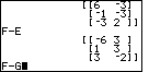
Here the calculator has informed us that the problem F-G is not legal.
As we examine the two matrices we see that F is a 2x3 matrix and
G is a 3x3. They are not of the same order. Therefore, subtraction
is not defined for these two matrices. We press
to select option 5, QUIT, from the menu.
|
| Problems 22 and 23 are shown in Figure 44. |
|
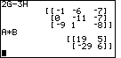
Problems 24 and 25 are shown in Figure 45, along with the statement of problem 26.
Problem 25 shows a new operation for matrices. This operation is called
scalar multiplication. In scalar multiplication we multiply
a matrix by a number. Problem 25, 2A,
can be placed into the calculator by pressing
.
The calculator recognizes the "implied" multiplication. This was done in Figure 45.
We could have used the multiplication button,  ,
between the 2 and the A.
We would still have a case of scalar multiplication. ,
between the 2 and the A.
We would still have a case of scalar multiplication.
An examination of the answer for problem 25 shows how scalar multiplication works. Each element of the matrix is multiplied by the scalar number. Note the difference between scalar multiplication and the elementary row operation of multiplying a row by a number. These are quite different operations. |
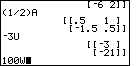
| Figure 46 continues the demonstration of scalar multiplication for problems 26 and 27, along with the statement of problem 28. We see an example of multiplying by a scalar fraction and by a negative scalar. |
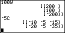
| Figure 47 continues the demonstration of scalar multiplication for problems 28 and 29. |
| Figure 48 continues the demonstration of scalar multiplication for problem 30. Then, Figure 48 demonstrates the combination of matrix subtraction and scalar multiplication with problem 31, A-2B. We need to examine that result and see that it comes from taking each element of A and subtracting twice the value of the corresponding element of B. |
| Figure 49 has another successful example in showing problem 32 with its answer. The screen concludes with a statement of problem 33. As we remember the order of matrices D and F (namely, 2x3 and 3x2, respectively) we should expect that problem 33 will cause an error. |
|
|
Figure 50 verifies our prediction. Scalar multiplication does not change the order
of a matrix, and we know that we can not subtract matrices of different orders.
Again, use
to select option 5, QUIT, from the menu on Figure 50.
|
| Problems 34 and 35 are shown in Figure 51. |
|
Figure 52 starts with another example of combining scalar multiplication with
subtraction in problem 36, 2G-3H.
Figure 52 then demonstrates problem 37 which calls for the multiplication of two
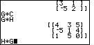
matrices. In the book the problem is written as AB, where we understand the
implied multiplication. The calculator recognizes names such as AB
as two character variables. Therefore, unlike scalar multiplication,
we need to use the multiplication symbol to indicate the operation.
We press |
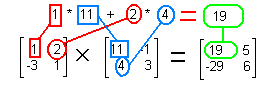
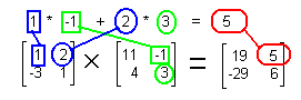
| Multiply row 1 of A times column 1 of B to get row 1 column 1 of the answer. |
| Multiply row 1 of A times column 2 of B to get row 1 column 2 of the answer. |
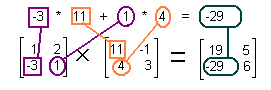
| Multiply row 2 of A times column 1 of B to get row 2 column 1 of the answer. |
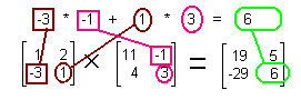
| Multiply row 2 of A times column 2 of B to get row 2 column 2 of the answer. |
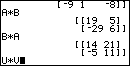
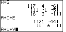
| In Figure 57 we can see one immediate consequence of our definition of matrix multiplication. In particular, Figure 57 shows both A*B and B*A. We can see that these two do not produce the same results. Whereas multiplication of numbers is commutative, in general, the multiplication of matrices is not commutative. Figure 57 ends with a statement of problem 39. |
|
| Unfortunately, pressing the key at the
end of Figure 57 produces that error message again. What is wrong? We know
that we can add U and V because they have the same order. Why can't we
multiply them?
When we multiply matrices the number of columns of the left matrix must match the
number of rows of the right matrix. In Figure 57,
for A*B and B*A
this was not a problem since these are square matrices and both have
2 rows and 2 columns. But U is a 2x1 matrix and so
is V. Thus, U has 1 column, but
V has 2 rows. Matrix multiplication is not defined
in such a case. We press
|
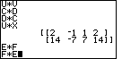
| Figure 59 shows the next few problems. Problem 40, CD, does not work because the 3 columns of C do not match the 2 rows of D. Problem 41, DC, does not work because the 3 columns of D do not match the 2 rows of C. Problem 42, UX, works since the 1 column of U matches the 1 row of X. It is worth your time to verify this multiplication by hand. Problem 43, EF, does not work because the 2 columns of E do not match the 3 rows of F. Problem 44 is stated but not executed until Figure 60. |
| Figure 60 shows that problem 44 does not work, as expected, but that we can do problems 45, and 46. Problem 47 is stated but not performed. In fact, the result of problem 47 was accidentally omitted from the screen captures. However, we know that C is a 2x3 matrix and U is a 2x1, so the product is undefined, because the 3 does not match the 2. |
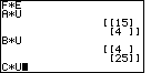
| On the other hand, problem 48 asks for C*W, where C is 2x3 and W is 3x1. This works, and the answer is in Figure 61, as is the answer for problem 49. |
| Figure 62 contains the solutions to problems 50 and 51. |
| Figure 63 shows that problems 52 and 53 do not work, but 54 does. |
| Figure 64 shows problem 55 failing, but 56 working. |
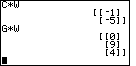
| Figure 65 should be used with Figure 64 as a further demonstration that matrix multiplication is not commutative. The answers for G*H and H*G are very different. Since these matrices are square, the product is defined for both problem 56 and 57. Figure 65 also shows the beginning of some work on problem 58. That problem did not ask us to actually multiply the matrices, but it is nice to see that the calculator has no problem doing just that. |
| Figure 65 continues the work on portions of problem 58. Knowing that the multiplications work, it is worth the time to go through these and make sure that you could predict the size of the answer from the sizes and order of the original matrices. |
There are many other details of matrices that are not covered in this set of examples. The course notes will be updated to point out the details that are considered to be of highest importance.
©Roger M. Palay
Saline, MI 48176
February, 1998
