

|
This demonstration starts with a calculator that has no defined matrices.
We have used the   keystrokes to open the MATRIX window. Then we use the
 twice to move to the EDIT option.
Finally we press twice to move to the EDIT option.
Finally we press  to move to edit the highlighted
matrix, matrix [A]. to move to edit the highlighted
matrix, matrix [A].
|
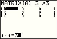 |
Here we have already pressed
   to set the dimensions of the matrix so that it has 3 rows and three columns.
|
 |
In Figure 3 we have entered all of the elements of the desired matrix
although we have yet to press the  key to accept the final value, namely 5, for the third row
third column entry. We move to Figure 4 by pressing the
 key and then we exit the
MATRIX EDIT window by
pressing key and then we exit the
MATRIX EDIT window by
pressing   . .
|
 |
Again, this calculator started with nothing on it so we are back at a blank screen.
We would like to see the contents of [A] so we will return to
the MATRIX window via the keys
  . .
|
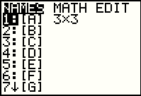 |
Not to belabor the point, but to get the name of a matrix onto the main screen we need to use the MATRIX menu to select the
name of the matrix. The calculator does not recognize [A]
as the name of a matrix if we type it as three separate characters.
Given that our desired matrix is already highlighted in Figure 5
we need only press  to select the name of that
matrix. to select the name of that
matrix.
|
 |
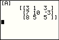
In FIgure 6 we have the result, the name of [A] pasted ontot he screen.
We press  to tell the calculator to evaluate
the command, which it does and displays in Figure 7. to tell the calculator to evaluate
the command, which it does and displays in Figure 7.
|
 |
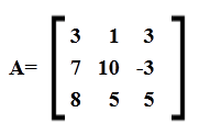
Here we see the original matrix. Unfortunately for us, the algorithm for determining the inverse of
this matrix requires that we start with a matrix that has this
as its first three columns and the identity matrix as its last three columns.
what we really want is
 |
 |
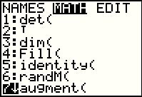
The first command that we want is the augment( command, found in
the MATRIX MATH screen. Press   and
and  to get to the screen on Figure 8. The desired command is at the
bottom of the screen. to get to the screen on Figure 8. The desired command is at the
bottom of the screen.
|
 |
We use the  key to move the highlight to the desired command.
Then use the key to move the highlight to the desired command.
Then use the  key to select that command and paste it to the screen. key to select that command and paste it to the screen.
|
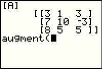 |
The augment( command takes two arguments, both matrices, and it produces a new matrix by "pasting" the two matrices together. We return to the MATRIX menu to select the name [A] from the list of the matrices (Figure 5 has the screen that we would use). |
 |
Now, the second argument needs to be a 3x3 identity matrix. We can manufacture such a matrix by using the identity( command. Return to the MATRIX MATH menu to find that command. |
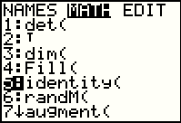 |
Figure 12 shows the MATRIX MATH menu and has the correct function highlighted.
Press  to past the command onto the main screen. to past the command onto the main screen.
|
 |
The command is almost complete. We still need to tell the identity( command the size of the desired identity matrix. |
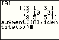 |
Figure 14 has the completed command. The 3 indicates that we want a 3x3 identity matrix. The first right parenthesis, ), ends the identity( command. The final right parenthesis ends the augment( command. |
 |
Pressing the  key to perform the command
produces the matrix shown in Figure 15. This is the matrix that we want.
It is stored in the Ans location. key to perform the command
produces the matrix shown in Figure 15. This is the matrix that we want.
It is stored in the Ans location.
The goal, for the next number of steps, will be to use the elementary row operations to convert the first three columns of the augmented matrix into the identity matrix. There are many ways to do this. In this case we will start the process by swapping the first two rows. |
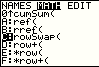 |
To do this we return to the MATRIX MATH menu, and move down
to the rowSwap( command. Then press  to select that command.
|
 |
The syntax of the rowSwap command is to specify the matrrix to use, followed by the numbers of the two rows to use. |
 |
We use the   key
sequence to generate the Ans name, and then follow that by
the rest of the command. key
sequence to generate the Ans name, and then follow that by
the rest of the command.
|
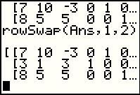 |
The row swap is complete. Now, to generate a 1 in row 1 column 1 we want to multiply row 2 by -1 and add it to row 1. The command to do this is the *row+( command. |
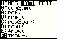 |
Figure 20 is a return to the MATRIX MATH menu were we have moved to highlight the *row+( command. |
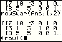 |
Press  to past the command ontop the screen.
The syntax of the *row+( command is to specify the
number to use to multiply the row,
then the name (location) of the matrix to use, and finally,
the numbers of the rows to use. to past the command ontop the screen.
The syntax of the *row+( command is to specify the
number to use to multiply the row,
then the name (location) of the matrix to use, and finally,
the numbers of the rows to use.
|
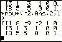 |
Figure 22 shows both the completed and the executed command. We now have the desired 1 in row 1 column 1. The next step is to get a 0 in row 2 column 1. We can do this by multiplying -3 times row 1 and adding the result to row 2. |
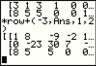 |
Figure 23 shows the needed command and the result of executing it. Now that there is a 0 in row 2 column 1, the next step is to get a 0 into row 3 column 1. We do that by multiplying -8 times row 1 and adding the result to row 3. |
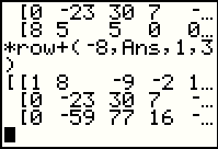 |
Figure 24 shows the desired command and the result.
Our next step is to generate a 1 in row 2 column 2. As before, there are many ways to do that. We will spend the next few steps doing this without generating any fractions. (If you want to do this in a more direct way, using fractions, skip down to Figure 38.) To do this without generating fractions we need to find a multiple of 23, the value in row 2 column 2, and a multiple of 59, the value in row 3 column 2, that are different from each other by 1. We observe (after a lot of examination) that 18*23 is 414 and 7 times 59 is 413. We can use these to get our desired result. First we multiply row 2 by -18 to generate a 414 in row 2 column 2. |
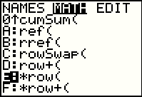 |
The command that we want to use is *row( command. We return to the MATRIX MATH menu to find that command. |
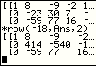 |
The syntax for the *row( command is to give the value used to multiply, the name of the matrix to use, and finally the number of the row to multiply. You can see the completed command and the result of the command in Figure 26. |
 |
Having performed the command in Figure 26 we are ready to multiply 7 times row 3 and add it to row 2. Figure 27 shows that command and the result. As you cn see, our objective, to get a 1 in row 2 column 2 has been accomplished. The next stepis to get a 0 into row 3 column 2. |
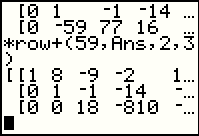 |
Multiplying row 2 by 59 and adding the result to row 3 generates the desired 0.
The next step is to generate a 1 in row 3 column 3. This time we have no choice but to multiply row 3 by 1/18. |
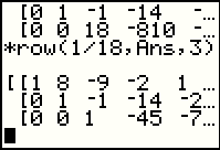 |
The command to multiply row 3 by 1/18 is shown in Figure 29.
The result has the desired 1 in row 3 column 3.
At this point we have generated 1's down the main diagonal and we have 0's below that diagonal. In the process of generating this situation, we have also generated new values in columns 4, 5, and 6. We can see some of those values in Figure 29, but we might want to examin the rest of the matrix. |
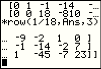 |
To do this we use the  key repeatedly to move the display to the right.
The result appears in Figure 30.
|
 |
Our next phase will be to generate 0's above the diagonal, starting in column 3. However, since we already have 1's on the main diagonal, this is a straight forward task. We start by working up column 3. Multiplying 1 times row 3 and adding it to row 2 will generate the desired 0 in row 2 column 3. |
 |
Multiplying 9 times row 3 and adding it to row 1 will generate the desired 0 in row 1 column 3. |
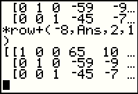 |
Having completed column 3, we move back to column 2.
Multiplying -8 times row 2 and adding it to row 1
will generate the desired 0 in row 1 column 2.
After performing the command, the right side of the matrix holds the desired inverse of the original matrix. In Figure 33 we can only see part of that answer. |
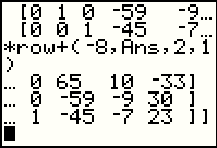 |
To get to Figure 34 we have used the cursor control key to move the display to the right.
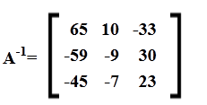
There is our answer. The inverse matrix is
 |
 |
Unfortunately, there is no easy way to chop apart a
matrix the way we assembled on, back in Figures 14 and 15.
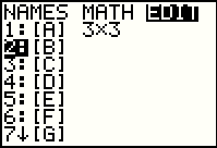
We will have to re-enter the matrix, this time as [B].
To do this we return to the MATRIX EDIT menu and highlight option 2, [B].
Then press  to start the editor for [B]. to start the editor for [B].
|
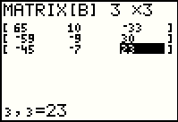 |
In Figure 36 we have entered the desired dimensions and values for the inverse matrix.
Once wew are done we
press   to exit the editor.
|
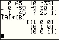 |
Figure 37 reflects our construction of [A]*[B]
along with the result of pressing the  key
to perform the multiplication. As you see, the result is indeed the
3x3 identity matrix. key
to perform the multiplication. As you see, the result is indeed the
3x3 identity matrix.
|
 |
For the sake of completeness, Figures 38 through 49 redo some of the work that we already did, but this time avoiding the strange multiplication that we did in Figure 26. Figure 38 shows the matrix as it existed before that multiplication. Our task, at this point in the proces was to get row 2 colum 2 to be a 1 instead of its current value of -23. |
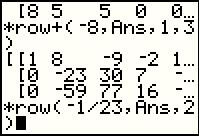 |
The most straight forward command to do this is to multiply row 2 by -1/23. The command to do this is shown at the bottom of Figure 39. This will work, but it will also generate fractional values which will be displayed as decimal values if we perform the command as written. |
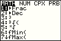 |
We open the MATH menu by pressing the  key.
The first option is the one we want.
Press key.
The first option is the one we want.
Press  to paste that option to the end of the command
that we started in Figure 39. to paste that option to the end of the command
that we started in Figure 39.
|
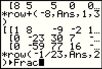 |
Here is the complete comamnd. Press  to perform the comamnd
and move to the next Figure. to perform the comamnd
and move to the next Figure.
|
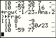 |
Indeed, we have created the 1 in row 2 column 2, but we have introduced fractions in the rest of row 2. |
 |
Figure 43 shows the right sidee of the matrix, displaying more of the fractional values. |
 |
Having the 1 in row 2 column 2, the next step is to generate a 0 in row 3 column 2. The command to do this and the result of performing that command is shown in Figure 44. |
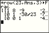 |
To convert the -1/23 in row 3 column 3 to a 1, we multiply that row by 23. |
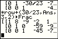 |
To convert the -30/23 in row 2 column 3 to a 0, we multiply row 3 by 30/23 and add the result to row 2. |
 |
To convert the -9 in row 1 column 3 to a 0, we multiply row 3 by 9 and add the result to row 1. |
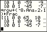 |
To convert the 8 in row 1 column 2 to a 0, we multiply row 2 by
-8 and add the result to row 1.
Having done all of this we have achieved our goal with teh identity matrix now in columns 1-3 and the inverse in columns 4-6. In Figure 48 we can see just part of the inverse matrix. |
 |
For Figure 49 we use the cursor control key to move the display to the right. |
 |
As much fun as is the process for finding the inverse, it really is a bit tedious.
Fortunately, the calculator is willing to do all of this behind the scenes.
If we use the MATRIX menu to paste [A] onto our main screen, and follow that by
using the  key to generate -1
and then put the command to display the result in fractional form after that,
then press key to generate -1
and then put the command to display the result in fractional form after that,
then press  , the calculator respondes directly with Figure 50
giving the inverse matrix. , the calculator respondes directly with Figure 50
giving the inverse matrix.
|
 |
All of the work that has been done so far has been on our original matrix.
That matrix is a somewhat special case in that its matrix does not have fractional
values. A more common case is that when all of the elements in the origianl
matrix are integers, then the inverse matrix will contain fractional values.
To demonstrate this, Figure 51 returns to the MATRIX EDIT screen to change the value of
just one element of our original matrix.
Originally, the value in row 1 column 1 was a 3.
We have used the editor to change that value to be 4.
Press the   sequence to exit the editor.
|
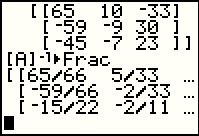 |
To generate the command on Figure 52 it was
enough to recall the last command via the
  sequence.
Then, use the sequence.
Then, use the  key to
perform the command. The result, shown in Figure 52 has
many fractional values in the inverse. key to
perform the command. The result, shown in Figure 52 has
many fractional values in the inverse.
|
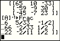 |
Figure 53 merely shows the rest of the inverse from Figure 52. |
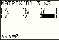 |
Finding the inverse is not always so easy. In Figure 54 we have created a new matrix, this time stored in [D]. |
 |
Here we have displayed the matrix and formulated the command to
find the inverse matrix. Press the  to move to Figure 56.
|
 |
Figure 56 shows that there is an error here. The error is designated as SINGULAR MAT. This means that there is no inverse. We have the same situation with numbers, namely that there is no inverse for the number 0. With matrices, however, it is possible for a matrix such as [D] that is not the zero matrix to still not have an inverse. |
 |
We conclude this page by showing yet another matrix, this one not having any 0 in it, that has no inverse. |
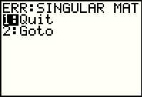 |
Indeed, the calculator reports that our matrix [E] is SINGULAR, and therefore has no inverse. |
©Roger M. Palay Saline, MI 48176 February, 2011