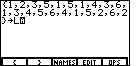
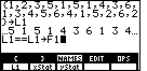
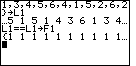
| xStat | 1 | 2 | 3 | 5 | 1 | 5 | 1 | 4 | 3 | 6 | 1 | 3 | 4 | 5 | 6 | 4 | 1 | 5 | 2 | 6 | 2 |
| yStat | 1 | 1 | 1 | 1 | 1 | 1 | 1 | 1 | 1 | 1 | 1 | 1 | 1 | 1 | 1 | 1 | 1 | 1 | 1 | 1 | 1 |
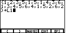
On the other hand, we could have examined the original data and we could have noted that there are only six different values in the data set, namely, 1, 2, 3, 4, 5, and 6. We could have counted the number of times each value appears in the data set. For example, the value 1 appears 5 times in
| xStat | 1 | 6 | 2 | 4 | 5 | 3 |
| yStat | 5 | 3 | 3 | 3 | 4 | 3 |
Our approach here will be to use the first representation, namely,
| xStat | 1 | 2 | 3 | 5 | 1 | 5 | 1 | 4 | 3 | 6 | 1 | 3 | 4 | 5 | 6 | 4 | 1 | 5 | 2 | 6 | 2 |
| yStat | 1 | 1 | 1 | 1 | 1 | 1 | 1 | 1 | 1 | 1 | 1 | 1 | 1 | 1 | 1 | 1 | 1 | 1 | 1 | 1 | 1 |
Now that we have determined the representation, the next question is "How do we create xStat and yStat, and how do we get the right values into them?" xStat and yStat are always on the TI-85 calculator. We do not need to create them. However, we do need to put the desired values into these two lists. The TI-85 allows us to edit these lists, to change the values in them, to add new values into the lists, and to delete values from the lists. We will return to this feature later. Our first approach will be to create two lists, separate from xStat and yStat, and then to copy those lists to xStat and yStat.
Make sure that the calculator has been turned on (press the
![]() key), and it
might be a good idea to start with a clear screen (press the
key), and it
might be a good idea to start with a clear screen (press the
![]() key).
key).
|
In order to create a list we will need to be able to
use the left brace, {, and the right brace, }. These
characters are not on the keyboard. We press the
|
| We want to start our list with a left brace, {.
Therefore, press the |
| A LIST is
a sequence of numbers separated by the comma character. Our list is the values in
the data set. Therefore, we enter the values one after the other, just as they were
given, and place a comma between values.
The key sequence is


 .
We conclude the LIST with a right brace, selected from the menu by
pressing the
.
We conclude the LIST with a right brace, selected from the menu by
pressing the
 key. This should leave the screen
as in Figure 3. key. This should leave the screen
as in Figure 3.
|
|
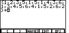
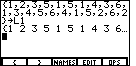
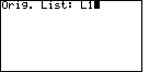
In Figure 3 we have constructed a LIST.
However, we want to save that LIST.
To do this we need to store the list.
We press the  key to paste the "store" symbol,
 |
|
We store the list to a variable. We get to make up the name for that variable.
In this example we will store the list to a variable called L1.
Variable names need to start with a letter,
and then they can be up to eight characters
long, using letters and digits.
To get the
"L" we press the  key. This will produce
Figure 5. Now, to complete the name we need to
shift out of ALPHABETIC MODE. key. This will produce
Figure 5. Now, to complete the name we need to
shift out of ALPHABETIC MODE.
|
| Press the  key shift out
of ALPHABETIC MODE and then press the
key to generate the "1",
as in Figure 6. key shift out
of ALPHABETIC MODE and then press the
key to generate the "1",
as in Figure 6. |
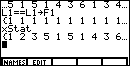
| Through Figure 6 we have constructed a list and formulated
the command to store it in a variable called L1. However, we have not told
the calculator to perform those actions. We do this by pressing the
 key.
The calculator responds by displaying the new list. Note that there are
no commas in this displayed list. Furthermore, the list runs off the screen,
with three dots, ..., following the 6. Those dots indicate that there is
more to the list. We can see more of the list by pressing the key.
The calculator responds by displaying the new list. Note that there are
no commas in this displayed list. Furthermore, the list runs off the screen,
with three dots, ..., following the 6. Those dots indicate that there is
more to the list. We can see more of the list by pressing the
|

| Figure 8 shows the result of having pressed the
|
| For Figure 9 we have pressed
the  key to open a submenu that
gives all of the LISTS currently defined in the TI-85 calculator. key to open a submenu that
gives all of the LISTS currently defined in the TI-85 calculator.
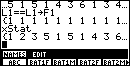
Note that the calculator used to produce Figure 9 has three lists defined, L1, xStat, and yStat. Your calculator may have other lists defined. You may need to press the MORE key to shift the submenu until you can see the L1 list. Even then it might not be in the first position. The discussion below is based on having L1 in the first position. |
| We want to form the expression L1= =L1
and then store that new list in F1.
We could type all of this, but we will take the shortcut of using the name L1
from the submenu. Thus, we press
 to paste L1 on the screen,
to paste the first equal sign,
to paste the second equal sign,
to paste L1 ,
to paste to paste L1 on the screen,
to paste the first equal sign,
to paste the second equal sign,
to paste L1 ,
to paste  to paste the "F", and finally
to paste the 1.
That should leave the screen of the
calculator as in Figure 10.
to paste the "F", and finally
to paste the 1.
That should leave the screen of the
calculator as in Figure 10.
|
|
Again, in Figure 10 we formulated the command. We press the
key to tell the calculator to perform the
command. We have done that in Figure 11 and the result shows the new list of twenty-one
1's.
|

| We are done with the LIST menu and the NAMES submenu shown in Figure 11.
We can close those menus by pressing the
 to close the submenu, and the
key again to close the LIST menu. That leave the display as in Figure 12.
to close the submenu, and the
key again to close the LIST menu. That leave the display as in Figure 12. |
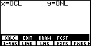
| For Figure 13 we open the STAT menu by pressing the
 key. Of the five displayed options, we want to select
the first option, CALC. To do this we press the
key, which will move us to Figure 14. key. Of the five displayed options, we want to select
the first option, CALC. To do this we press the
key, which will move us to Figure 14.
|
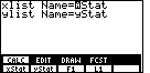
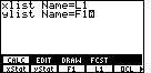
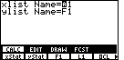
| Figure 14 gives the default configuration. The calcualtor is looking for two lists of numbers, the xlist and the ylist. By default the calculator believes that the xlist should be in xStat, and that the ylist should be in yStat. We, on the other hand, have placed our xlist, the list of values, into the variable L1. In addition, we have placed the corresponding frequency list in F1. Fortunately, selecting the CALC option has not only displayed the default configuration, it has also displayed a new submenu giving the names of the defined LISTs on this calculator. (Note that both L1 and F1 appear in that submenu.) |
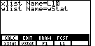
| The calculator was waiting with the default configuration, with the
cursor in position for us to give a replacement name for xStat
as the source for the xlist. We need only press
the  to select L1 from
the submenu and paste it into that position.
Figure 15 reflects this action. to select L1 from
the submenu and paste it into that position.
Figure 15 reflects this action.
|
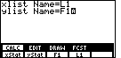
| We accept the new name for the xlist, as given in Figure 15, by pressing the
key. That will move the cursor to
the next line to specify the ylist.
Again, we replace the default value, yStat, with the name F1, which
we can select from the submenu by pressing the
key.
|
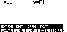
| We leave Figure 16 and move to Figure 17 by pressing the
key. Notice that this action changes the
submenu, providing us with new options.
|

| Figure 18 shows the result of pressing
the key to select the 1-VAR option from
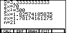
the submenu. Figure 18 has the first results tht we wanted to compute. The TI-85
has computed six different values for the numbers in our data set. The first value,
The second line, The fifth value, The final output line, |
| We close the submenu of
Figure 18 by pressing the key.
|
| We close the menu of Figure 19
by pressing the key again. This
leaves us with Figure 20.
|
| Now we will move to open the LIST
menu by pressing the 
 keys.
Then we press
to open the submenu that shows the names of the lists in the calculator.
On the calculator used here there are only four lists, F1, L1,
xStat,
and yStat. keys.
Then we press
to open the submenu that shows the names of the lists in the calculator.
On the calculator used here there are only four lists, F1, L1,
xStat,
and yStat.
|
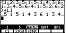
| We can see the contents of xStat by pressing
the
key to
select the third option from the submenu and paste it onto the screen.
|
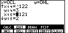
| In Figure 22 we had pasted xStat onto the screen.
Now we press to tell the calculator to display
the contents of xStat. Figure 23 shows us that xStat
hold a copy of the the values that we had put into L1. We did a
statistical analysis earlier, in Figures 17 and 18. In doing that, the calculator
automatically copies the list identified as the xlist to xStat, and it
copies the list identified as the ylist to yStat. Then, the calculator
does the statistical operations using xStat and yStat.
|
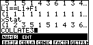
Figures 19 through 23 confirm that we did use xStat and yStat. Now we will turn our attention to finding the median and the mode of the data. Unlike the finding the mean, the TI-85 does not have a built-in process for finding the median and the mode. We have a program written for the TI-85 that will help in finding these values. That program is called COLLATE3. You can get a copy of the program from another TI-85 that has it, or you can use the TI-Graph Link program to transfer COLLATE3 from a PC that is storing it. The page collate3.htm holds a listing of the program (in case you want to type it into your calculator) and it has a link that will allow you to download the program to a PC (for subsequent transfer via TI-Graph Link).
| We start by pressing the  key
to open the PROGRAM menu. Here we have two options, NAMES to list the names of the
programs, and EDIT to edit the programs, that is to change them.
We want to see the names. key
to open the PROGRAM menu. Here we have two options, NAMES to list the names of the
programs, and EDIT to edit the programs, that is to change them.
We want to see the names.
|
| Press the key to display the
NAMES submenu. The calculator used to generate Figure 25 has a large number
of programs. They are listed in alphabetic order. COLLATE3 is not among those
listed in Figure 25. However, the |
| We press the  key
to shift the submenu display to show more names.
The new submenu is shown in Figure 26.
Although COLLATE3 is not shown, we do see COLLA as the second item in the
submenu. The submenu only shows us the first four or five characters of each name.
Therefore, the second option is the one that we want to select.
We press
to select that option. The calculator
pastes COLLATE3, the full name of the program, onto the screen. key
to shift the submenu display to show more names.
The new submenu is shown in Figure 26.
Although COLLATE3 is not shown, we do see COLLA as the second item in the
submenu. The submenu only shows us the first four or five characters of each name.
Therefore, the second option is the one that we want to select.
We press
to select that option. The calculator
pastes COLLATE3, the full name of the program, onto the screen.
|
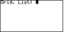
| To start the program we simply press the
key. The first thing that the
COLLATE3 program does is clear the screen. Then it asks us for the Original List of
values. Our original list was stored in L1. We will need to supply that
name in response to this question.
|
| We could open the LIST menu and display the names of the
lists and then select the one we want to paste onto the
screen. However, in this case, we might
as well just enter the name. We can enter the name L1 by
pressing the key to indicate that
the next key should be alphabetic, pressing the
key to select L, and then pressing the
key to produce the 1. The result is
shown in Figure 28.
|
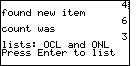
| We press the key to accept the
name supplied in Figure 28. The calculator will produce numerous lines of output
until it pauses as shown in Figure 29. At this point the calculator has done much
of its analysis and work. It is waiting to show us the results.
|
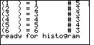
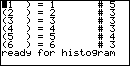
| We press to have the calculator continue
with its output. Figure 30 shows us the output. This output is given as three columns
of values. The first column will always start with 1 and increase by 1 for each line of
output. This first column is counting the different values found in our data set.
The second column displays the different values found in the data set. These values
will be sorted from lowest to highest. The second column in Figure 30 indicates that we have values
in the data set ranging from 1 through 6. The third column of the data set indicates the
number of times each item in the second column appears in the data set. Thus, we see that
the value 1 appears 5 times, that 2 appears 3 times, and so on.
We can examine the second and third columns to find the mode value of the data set. The mode will be the value in the second column that corresponds to the largest value in the third column. In Figure 30, 5 is the largest value in the third column. Therefore, the mode of the data set is 1, the value of the second column that corresponds to the 5 in the third column. We can also use the output of Figure 30 to find the median. Remember that the median is the middle value in the sorted data values. We remember, from Figure 18, that there were 21 values in our data set. That means that if we sort the values, then we want the 11th value (it will have 10 values that are less than or equal to it and 10 that are greater than or equal to it). From Figure 30 we see that there are 5 1's, 3 2's, and 3 3's. Therefore, the 11th value is a 3, which makes the median of the data set be 3. [We will see another way to find the median in the second example.] |

| Figure 30 shows the output of the COLLATE3 program.
However, that program is not quite done. (We can see that the program is merely paused,
not completed, by the small vertical line of dots at the upper right of the
display in Figure 30.)
We press to continue the program.
COLLATE3 concludes by giving a graphic display of the input data in
terms of a histogram.
|
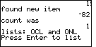
Figures 24 through 31 demonstrated the use of the COLLATE3 program. We will return that program in the second example data set below for a more complete illustration of the output. However, Figure 29 had some information that was not explained at that time. In particular, Figure 29 included a reference to two new lists, OCL and ONL. We will take a moment to examine these lists, which are produced by the COLLATE3 program.
| To move to Figure 32 we need to close the
histogram. We do this by pressing the key.
Note that Figure 32 returns to the display from before the histogram, essentially
Figure 30, but that the cursor is now in the top left corner on the screen.
Any work that we do will be writing over the existing screen.
|
| To view the new lists we will open the LIST menu by pressing
and then we will select the
NAMES option by pressing the
key. The result is shown in Figure 33.
|
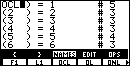
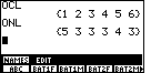
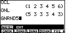
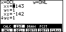
| The calculator used here shows a number of lists as
being defined. In this case, we want to look at OCL which is the
third item in the submenu. Therefore, press
to paste OCL onto the screen.
As expected, it appears in the upper left corner of Figure 34.
|
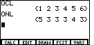
| We press to tell the calculator to
display the contents of OCL. In Figure 35, the contents of OCL
appear at the right side of the second line of the display.
The other material on the screen is just too distracting. We need to clear
the screen and do this again.
|
| Let us clear the screen by pressing the
|
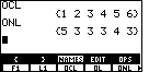
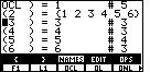
| Then we can display both the OCL and the ONL lists
by pressing
 .
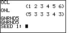
Looking at the output we can see that COLLATE3 creates OCL and ONL to
hold the different values that it finds and the frequency with which each value
appears. As you may recall, from the start of this document, the TI-85
can actually use that arrangement of data to compute the statistical values for
the mean and population standard deviation.
We will return to the statistics features and recalculate those values based on
these newly created lists.
.
Looking at the output we can see that COLLATE3 creates OCL and ONL to
hold the different values that it finds and the frequency with which each value
appears. As you may recall, from the start of this document, the TI-85
can actually use that arrangement of data to compute the statistical values for
the mean and population standard deviation.
We will return to the statistics features and recalculate those values based on
these newly created lists.
|
| We open the STAT menu by
pressing the key.
|

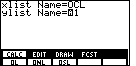
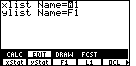
| From the Stat menu we select the first option, CALC, by
pressing the key. The calculator responds
by asking for the xlist and ylist. (Note that the default values are the ones that
we last used.) In this case we want to change those assignments so that
xlist is OCL and ylist is ONL.
|
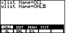
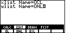
| It is easy to paste OCL into position for the
xlist. We need only press and
to select OCL from
the submenu. In order to find ONL we will have to press the
key to display more lists.
Those actions produced the screen shown in Figure 40.
|
| Figure 41 shows the completed update for xlist and ylist
as a result of pressing to select ONL
for the ylist.
|
| We can accept the changes made in Figures 40 and 41
by pressing the key.
In Figure 42 we are ready to perform the statistical analysis.
|
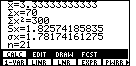
| We press to select the 1-VAR
option in the submenu of Figure 42. This produces the output seen in
Figure 43. Note that Figure 43 is the result of doing the statistical analysis
on the two lists OCL and ONL.
Figure 19 was the result of doing the statistical analysis on the two lists L1 and F1
A comparison reveals that Figure 19 and Figure 43 are identical, which is what we should have
expected. Note that the value of |
The first 43 Figures demonstrate statistical processing for a 21-element data set. It is nice to see the TI-85 do all of the computations, but the process seems to take many steps just to process those 21 values. The real power of the TI-85 can be seen if we look at processing a much larger set of data. For example, consider the following table of numbers taken from a sample test on this material.
| -113 | -133 | -132 | -91 | -123 | -121 | -93 | -103 | -104 | -102 | -106 | -126 | -136 | -90 | -120 |
| -105 | -140 | -125 | -127 | -110 | -109 | -109 | -128 | -88 | -114 | -133 | -143 | -120 | -97 | -108 |
| -102 | -107 | -96 | -108 | -91 | -115 | -122 | -122 | -82 | -111 | -130 | -116 | -97 | -122 | -107 |
| -85 | -135 | -116 | -116 | -94 | -91 | -142 | -119 | -119 | -121 | -115 | -117 | -120 | -136 |
We could process this data using exactly the same steps that we used before.
The first step will be to get this list into the calculator. Even that seems to
be a formidable task. However, in this case,
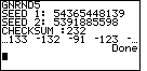
you can generate this same list on your calculator as
as L1 via the GNRND5 program on the TI-85
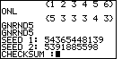
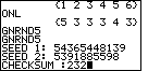
with
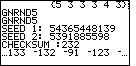
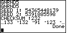
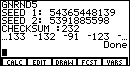
SEED 1=
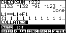
54365448139 and SEED 2= 5391885598 and CHECKSUM=232.
We will demonstrate using the program to do this.
| We move from Figure 43 to Figure 44 by pressing
and
to close first the submenu and then
the menu of Figure 43. Then we press
to open the PROGRAM menu, and we
press
to open the NAMES submenu. The program
that we want is not here. We will have to look at more of the submenu to find it.
|
| The calculator used here required us to
press and then press
again to shift the submenu to
the point where we could see GNRN (the abbreviation of GNRND5). Then we press
on this calculator to paste
GNRND5 onto the screen.
|
| Pressing the key will start the program.
In this case, the program prompts us to enter the value of the first seed.
|
| We supply the seed value by pressing the keys
to generate 54365448139 and then we press the
key to accept that value. The calculator then asks for the seed value. We enter the
digits for 5391885598 and press
to accept that value. The calculator
prompts for the CHECKSUM. Figure 47 shows all of this, with the calculator
waiting for us to enter the next value.
|
| In Figure 48 the checksum has been entered. |
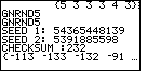
| We move from Figure 48 to Figure 49 by pressing the
key to accept the CHECKSUM value.
Assuming that we have correctly entered the two seed values and the CHECKSUM value, the
calculator will take a few minutes to actually generate a new list, stored in L1,
that has exactly the values given in the table above. When the calculator has
finished generating those values, it displays the new list, and it then waits for
us to press the ENTER key to finish the program. It waits in this condition so
that we can use the cursor arrow keys to examine parts of the list that do not fit on the screen.
In Figure 49 we see the first four values in the generated list. They correspond exactly to the first four numbers in the first row of the table given above. |
| We can see more of the values in the list if we press the
|
| Once we have examined enough of the list to
be sure that we have a copy of the data from the table, we press
to complete the program.
The calculator responds by writing the word Done at the right side of the screen.
|
The next few Figures (52 through 56) demonstrate a typical error. The small diversion is worth reading and examining.
| Now that we have created L1 we are ready
to move to the statistical analysis. We
open the STAT menu by pressing the key.
The menu appears as in the bottom of Figure 52.
|
| We select the CALC option from the
menu in Figure 52 by pressing the key.
Figure 53 shows the calculator responding with the
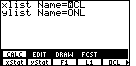
screen that associates the xlist and the ylist with our actual lists.
|
| We have generated Figure 54 by pressing
to paste L1 onto the screen,
to move to the next line, and
to paste F1 into the ylist spot.
|

| As before, we press
to accept our assignments. Now, with a new submenu we are ready to select the 1-VAR
option.
|
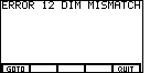
| At the end of Figure 55 we were ready to select the 1-VAR
option in order to have the calculator determine values such as the mean.
However, when we press to choose the 1-VAR
option, the TI-85 responds with Figure 56, informing us theat we have an error.
|
The problem in Figures 52 through 56 is that although we have a new list called L1 we are using the old F1 list. The new L1 has many more values in it than the 21 1's in the old F1. We need to go back and recreate F1.
| We can get out of the error message in Figure 56
by pressing to QUIT. That return us to
Figure 57.
|
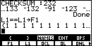
| In Figure 58 we open the LIST menu with
,
open the NAMES submenu with
,
select L1 with
,
paste two equal signs with the keys
,
select another L1 with
,
choose the "store" action via the
key,
select F1 with
,
and, finally, perform the action by pressing the
key.
The TI-85 does the calculation and displays the new F1, which
will have exactly as many 1's as there are values in L1.
|
| Now that we are ready to do the analysis, we open the
STAT menu via the key,
and we select the CALC option via the
key.
The TI-85 displays the default assignments to xlist and ylist.
These suit our needs.
|

| We have accepted those names by pressing the
key, and the
key.
|
| In Figure 60 we had the correct lists assigned to
xlist and ylist. We press
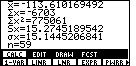
to perform the 1-VAR analysis. The result is given in Figure 61.
We can see that we had 59 values in the table, that the mean of those
values is – 113.610169492, and that the population
standard deviation is 15.1445206841.
|
| We have all the information that the built-in features
of the TI-85 will provide. Now we need to use the COLLATE3 program
to do some of the rest of the work. We press
to exit the submenu,
to exit the STAT menu,
to open the PROGRAM menu,
to open the NAMES submenu,
to shift that submenu so that we can see COLLA,
and
to paste COLLATE3 onto the screen.
|

| We start the program via the key.
The program clears the screen and asks for the name of the original list.
We enter it via
resulting in Figure 63.
|
| Again, press to
accept that name. The program spews forth line after line of output,
stopping when it is ready to move to the important output.
|
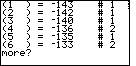
| We press to start that output.
Figure 65 shows the lowest 6 values that were in the original list and
the frequency with which each appeared.
|
| We press to get more of the values.
|
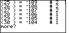
| Another shows the next set of 6 values.
We note here that – 122 and
– 120 were each found 3 times in the list.
|
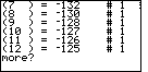
| Another shows more
values, and we can add – 116 to
the values that appear 3 time in the list.
|
| produces more values.
|
| Another to give 6 more values.
|
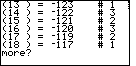
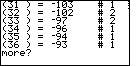
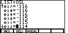
| And another shows the final 5 values.
Here – 91 ties the earlier mode
values by appearing 3 times in the original list.
We see that the mode values are – 122,
– 120, – 116, and
– 91.
|
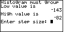
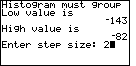
| In the earlier example, when the calculator stated that
it was ready for the the histogram we merely pressed the
ENTER key and the histogram appeared. Indeed, here
we press and the calculator
responds with Figure 72. The problem is that the program has been set to
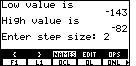
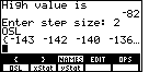
only do histograms that have 30 or fewer bars. Since the low value is
– 143 and the high value is
– 82, we must group values together to only have 30 or
fewer bars. The program is asking for the size of the groups.
|
| We choose to group values in intervals that are 2
wide. To do this we respond with .
|

| We accept our choice from Figure 73 by pressing
. The calculator produces the histogram.
|
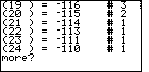
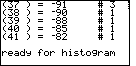
We have used the COLLATE3 program to find the mode values (see Figure 71). We could have written down our values from Figures 65 through 71 to find the median value, in line with our approach in the first example. However, there is an easier approach. We already know that COLLATE3 takes our original list and it produces new lists OCL and ONL. One may have noted, back in Figure 40, that COLLATE3 also produces a list called OSL. That list holds all of the values in the original list, but sorted from lowest to highest. We know that there are 59 values in the original list (see Figure 61). Therefore, the 30th item is the median value. The next Figures will demonstrate OSL and a method for displaying the value of the 30th item in that sorted list.
| First, we will exit the histogram display via
the key. Then we will
open the LIST menu via
, and the NAMES submenu via
.
|
| To find the OSL list we will need to use the
key to change the submenu.
On this calculator we choose the OSL list by using the
key. That will paste the name of the
list onto the screen. We press
to actually display the values in OSL.
|
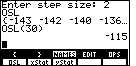
| We can have the calculator display a particular item in OSL
by following the name by the position number of the desired item,
enclosed in parentheses. Thus, we press
to paste OSL on the screen, followed by


 , and finally
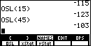
to display the value.
Figure 77 shows us that the 30th value in the sorted list is
– 115, so that must be the median value. , and finally
to display the value.
Figure 77 shows us that the 30th value in the sorted list is
– 115, so that must be the median value.
|
| For a 59 item list, such as our example,
the first quartile point will be in position 15 of the sorted list, and the third
quartile point will be in position 45 of the sorted list.
The key strokes to display these values are
, for the first quartile point; and
, for the second quartile point.
|
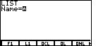
| We happen to have the LIST menu, and the NAMES submenu, displayed at the
bottom of Figure 78. We will use the EDIT option of the LIST menu to invoke the
LIST EDITOR. We can select that option via the keys
to indicate that we want to use the top
menu, and
to select the fourth item from the top menu, namely, EDIT.
The result is shown in Figure 79 where the calculator is waiting for us to
specify the name of the list that we want to edit.
|
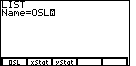
| We will need to press to shift the
list of names and then
to select the OSL name and paste it
into the desired spot.
|
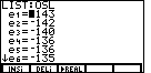
| Once we press to
move from Figure 80 to Figure 81, we are shown the items in OSL, one per line,
with an element number to the left of each item.
|
| We can move down the list by repeatedly
pressing the |
| Where the LIST EDITOR of Figures 79 through 82 was
helpful for looking at one list at a time, the STAT EDITOR is
used to look at a pair of lists. For us, we might want to return to
our lists OCL and ONL.
Figures 65 through 71 had shown us those pairs of values, but we might want to see them
again. We can exit from the LIST EDITOR of Figure 82 by pressing
. Then we open the STAT menu with the
key, and we select the EDIT option
by pressing the
key.
Again, the calculator wants to know which two lists it should use?
|
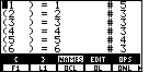
| For Figure 84 we selected OCL as the first list by pressing
and
. Then we moved to see more lists with the
key, where we selected ONL by using the
key.
|
| Pressing will start the
STAT EDITOR looking at our pair of lists. In this case each pair of x and y values is
listed, along with the corresponding list position number (the subscript).
|
| Again, we can move down the list by
repeatedly pressing the |
In summary, this page has demonstrated the use of the TI-85 calculator, along with an additional program or two, to find the mean, median, and mode of a set of numeric values. In the process we also found the range, the quartile points, and the population standard deviation.
©Roger M. Palay
Saline, MI 48176
January, 2000