Figure 1
| Figure 1 shows a blank HOME screen. If need be, you can press the
 key to move to this screen. key to move to this screen.
|
Figure 2
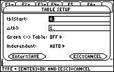
| We press the
  keys
to open the TblSet window.
The result is shown in Figure 2, although the highlighted area and values
may be different on a different calculators. Note that the calculator used to
generate Figure 2 had the value 0 under the blinking cursor. keys
to open the TblSet window.
The result is shown in Figure 2, although the highlighted area and values
may be different on a different calculators. Note that the calculator used to
generate Figure 2 had the value 0 under the blinking cursor.
The challenge from the openning paragraph was to look at the set of values
{-3, -2.5, -2, -1.5, -1, -0.5, 0}. To do this we want the
 value to be set at -3.
This will be the initial value in our table. value to be set at -3.
This will be the initial value in our table.
|
Figure 3
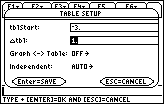
| We enter the desired value, – 3, into
the  area by pressing area by pressing
  . Then we
press . Then we
press
 to accept our value,and
  to
move the highlight to the next area.
This leaves the screen as is
shown in Figure 3. to
move the highlight to the next area.
This leaves the screen as is
shown in Figure 3. |
Figure 4
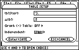
| With  set to -3, the next thing that we
want to do is to set the change from one value to the next. In our case, we want
the values to increase by 0.5.
We left Figure 3 with the highlight already on the set to -3, the next thing that we
want to do is to set the change from one value to the next. In our case, we want
the values to increase by 0.5.
We left Figure 3 with the highlight already on the
 field.
We set this field to be .5 by pressing the field.
We set this field to be .5 by pressing the
 and and  keys.
Then we can move the highlight down two fields by pressing keys.
Then we can move the highlight down two fields by pressing
  . This
is the state shown in Figure 4. . This
is the state shown in Figure 4. |
Figure 5
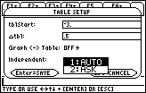
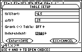
| The TABLE SETUP window shown in Figure 4 had the
Independent: value set at AUTO, and we had moved the highlight to
that field.
The Independent: field
controls how the calculator deals with the independent variable.
In our example, that is the x variable. This is the variable that will
take on the values that we select. The calculator will either determine these
values AUTOmatically, or it will ASK us for them.
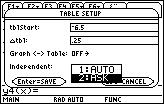
We can see these acceptable values by pressing the
 key. This brings up the selection
list shown in Figure 5.
We want to use the key. This brings up the selection
list shown in Figure 5.
We want to use the
 and and  settings to automatically generate independent values.
Therefore, we really do want to have the AUTO setting.
|
Figure 6

| We can reselect B from Figure 5 by pressing
 . Then we can accept and
save all of the new values on the window by pressing
the . Then we can accept and
save all of the new values on the window by pressing
the  key. This will return us to the HOME
screen shown in Figure 6. key. This will return us to the HOME
screen shown in Figure 6.
|
Figure 7
|
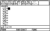
Now it is time for us to enter the
functions that we want to use in our table. To do this we will want to move to the
y= screen. We press
  to
change to the y= screen. to
change to the y= screen.
|
Figure 8
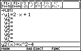
| We had two functions to evaluate,
y = 2x + 1
y = x2 – 4
Figure 8 shows the result of pressing
 
  to
generate the first function, to
generate the first function,
 to accept that first function and to get the calculator
ready to accept the second, and then
 
  to form the second function in the input area at the bottom of the screen.
|
Figure 9
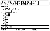
| All that remains is to press
 to accept that second function.
Doing so leaves the calculator as shown in Figure 9. to accept that second function.
Doing so leaves the calculator as shown in Figure 9.
|
Figure 10
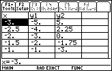
| After adjusting up the TABLE SETUP screen earlier, and now
defining the functions in Figure 9, we are ready to look at the table. To do
so we press
  .
In the first column, the
calculator displays values for the independent variable, x, starting with
our .
In the first column, the
calculator displays values for the independent variable, x, starting with
our  value, – 3,
and increasing by our value, – 3,
and increasing by our  value, 0.5.
The second column shows the corresponding values for the first function,
while the third column shows the corresponding values for the second function. value, 0.5.
The second column shows the corresponding values for the first function,
while the third column shows the corresponding values for the second function.
|
Figure 11
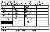
| We can move down the table by pressing
 
  to move the highlight as shown in Figure 11. It would appear, in Figure 11,
that the calculator has stopped the table after the highlighted entry.
There is a blank row beneath the highlighted row. In fact, the calculator is
merely waiting for us to move the highlight down one row, at which
point the calculator will compute new values for each of the three columns.
|
Figure 12
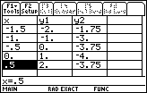
| In Figure 12 we have pressed
 
 to move the cursor down three rows, thus generating three
new sets of values. Note that we seem to have lost the old top rows. Figure
12 now has the value – 1.5 as its top value for x. to move the cursor down three rows, thus generating three
new sets of values. Note that we seem to have lost the old top rows. Figure
12 now has the value – 1.5 as its top value for x.
|
Figure 13
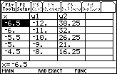
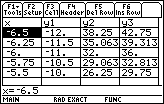
| As we might expect, we could press
 14 times to move the highlight
to new values at the top of the screen. Figure 13 reflects such a move,
forcing the top x value to be – 6.5 with appropriate new values
in the second and third columns. 14 times to move the highlight
to new values at the top of the screen. Figure 13 reflects such a move,
forcing the top x value to be – 6.5 with appropriate new values
in the second and third columns.
|
Figure 14

| Of course, we could press
  to return to the y= screen to allow us to define a new function.
We have done just that to generate Figure 14.
|
Figure 15
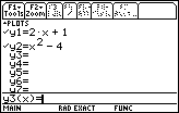
| Note that the highlight in Figure 14 was in the upper portion of the screen,
next to the y3= definition. By pressing the
 key, we direct the calculator to
move to the input line so that we can specify a new function. This is
shown in Figure 15. key, we direct the calculator to
move to the input line so that we can specify a new function. This is
shown in Figure 15.
|
Figure 16
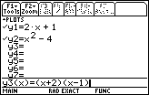
| Our new funtion will be
y3=(x+2)(x–1)
We enter that function by pressing


 and and  . .
|
Figure 17
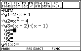
| To accept the funtion we press
 . The result is shown in Figure 17. . The result is shown in Figure 17.
|
Figure 18
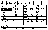
| When we return to the TABLE screen via the
  keys, the new functional values are displayed in the rightmost column.
|
Figure 19
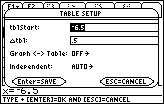
| The starting value for our independent variable, x,
in Figure 18 was – 6.5, exactly as we had left it in
Figure 13. In Figure 19 we use the
  keys to return to the TABLE SETUP window, where we can inspect the
current values. Note that the
 value is now
– 6.5, which reflects the current TABLE screen
values. As we scroll through the TABLE
the calculator adjusts the value associated with value is now
– 6.5, which reflects the current TABLE screen
values. As we scroll through the TABLE
the calculator adjusts the value associated with
 appropriately. appropriately.
|
Figure 20
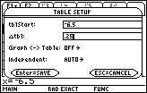
| Now that we are on the TABLE SETUP window, we can modify the
values before we return to the TABLE screen. In Figure 20 we have
pressed
 to move the highlight to the
 setting, and then we have pressed
  to generate a new value. to generate a new value.
|
Figure 21
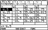
| We press  to
accept that value, and to
accept that value, and  to
save the current settings. This will cause us to return to the TABLE screen
shown in Figure 21. Note that the steps for the independent variable, x,
have been modified as we specified, and that new values for the three defined
functions are displayed. to
save the current settings. This will cause us to return to the TABLE screen
shown in Figure 21. Note that the steps for the independent variable, x,
have been modified as we specified, and that new values for the three defined
functions are displayed.
|
Figure 22
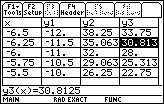
| One of the limittions of the TABLE screen is that the values in the
table are rounded to fit the available space. For example, we press
 
 and and  to
move the cursor to the second row of values in the rightmost column, shown in
Figure 22. In that "cell" the value 30.813 is highlighted. However, at the bottom of the
screen, in the input line, the
more precise value, namely 30.8125 is shown. to
move the cursor to the second row of values in the rightmost column, shown in
Figure 22. In that "cell" the value 30.813 is highlighted. However, at the bottom of the
screen, in the input line, the
more precise value, namely 30.8125 is shown.
Also, note in Figure 22, that the tabs at the top of the screen indicate that
the F4 key will perform the HEADER operation.
|
Figure 23
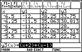
| If we press
 in Figure 22, the calculator responds with
Figure 23, where the function definition for the column holding the
highlighted cell, has been placed into the input line at the bottom of the screen. in Figure 22, the calculator responds with
Figure 23, where the function definition for the column holding the
highlighted cell, has been placed into the input line at the bottom of the screen.
|
Figure 24
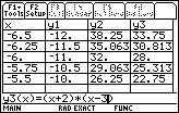
| We will change the function by editing it at this point.
We press
 to move the cursor to the
right end of the definition. Then press to move the cursor to the
right end of the definition. Then press  to move the cursor between the 1 and the ). Next,
press
  to remove the 1. And, finally, press
  to complete
the change to
(x+2)(x–3) to complete
the change to
(x+2)(x–3)
|
Figure 25

| Press
 to accept the new definition from the
input line of Figure 24 and return the screen to the TABLE, shown in
Figure 25. Note the new values in the rightmost column reflecting the
change in the function definition. to accept the new definition from the
input line of Figure 24 and return the screen to the TABLE, shown in
Figure 25. Note the new values in the rightmost column reflecting the
change in the function definition.
|
Figure 26
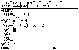
| In fact, if we return to the y= scrren via the
  keys, we can see, in Figure 26, that the actual definition of
y3 has been altered.
 |
Figure 27

| We will need to return to the TABLE SETUP window.
We do this by pressing the
 and and  keys.
Then we can move the highlight down to the Independent: setting by using the keys.
Then we can move the highlight down to the Independent: setting by using the
 
 keys. keys.
|
Figure 28

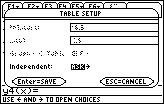
| We want to change the value of the Independent: setting.
We press
 to see the options, and
then to see the options, and
then  to highlight our desired choice,
ASK. to highlight our desired choice,
ASK.
|
Figure 29

| Press
 to make the highlighted choice of Figure 28 the
actual setting, as shown in Figure 29. Notice in Figure 29 that the old
values for to make the highlighted choice of Figure 28 the
actual setting, as shown in Figure 29. Notice in Figure 29 that the old
values for  and and  remain as a reminder, but that they are no longer available to us.
This is an indication that those values will not be used as far as maintaining the actual TABLE.
|
Figure 30

| We can press  to save the values set in Figure 29, and then
press to save the values set in Figure 29, and then
press
  to return to the TABLE screen, shown in Figure 30. We note that
although the TABLE values have not changed from the TABLE that we saw in Figure 25,
the "tab" choices at the top of the screen have changed.
We now have six options associated with our F1-F6 keys.
|
Figure 31

| The current TABLE is operating under the ASK setting.
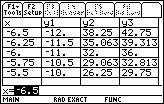
Therefore, we can change the values of the independent variable, x.
We do this by highlighting an x value, as we had in Figure 30, and then pressing the
 key.
Note that the highlight in Figure 31 has moved to the input line at the
bottom of the screen. key.
Note that the highlight in Figure 31 has moved to the input line at the
bottom of the screen.
|
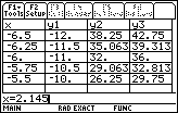
Figure 32

| We can change the value of the independent variable, x,
by entering a new value at this point. We press
 
 
 to enter the value 2.145. to enter the value 2.145.
|
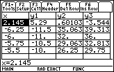
Figure 33

| We press
 to accept this new value and
to place it into the table.
Note, in Figure 33, that our value 2.145 has been inserted into
the TABLE, and that new values have been created for the three functions
defined for the next three columns. to accept this new value and
to place it into the table.
Note, in Figure 33, that our value 2.145 has been inserted into
the TABLE, and that new values have been created for the three functions
defined for the next three columns. |
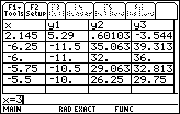
Figure 34

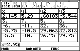
| To arrive at Figure 34 we press
 to move the highlight to the next
row, to move the highlight to the next
row,  to shift the highlight to the input line,
and to shift the highlight to the input line,
and  to enter the value 3. to enter the value 3.
|
Figure 35

| As before, we press
 to accept that new value, place it into the
TABLE, and cause new values to be computed for the other columns. to accept that new value, place it into the
TABLE, and cause new values to be computed for the other columns.
|
Figure 36

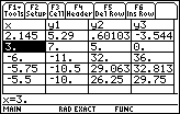
| Let us move to the last value in the table, – 5.5,
and change it to 3.01. We press
 
 to shift the highlight, to shift the highlight,
 to move to the input line, and to move to the input line, and
 
  to enter our new value.
|
Figure 37

| Pressing
 will complete the task started in Figure 36.
Now we will move to the open line at the bottom of the TABLE.
We do this by pressing
 . We
want to enter a new value in this spot. Therefore, we press . We
want to enter a new value in this spot. Therefore, we press
 to move the highlight
to the input line, and then to move the highlight
to the input line, and then 
 
 to enter our new value. This is
reflected in Figure 37. to enter our new value. This is
reflected in Figure 37.
|
Figure 38

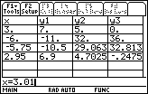
| In Figure 37 we had specified the new value, but we had not accepted it.
We press
 to accept that new value, as shown in Figure 38. to accept that new value, as shown in Figure 38.
|
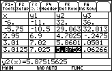
Figure 39

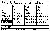
| For Figure 39, we move down to the open line
via the  key. Then we use
the key. Then we use
the  key to move to the input line.
We enter a new value, 3.0125, by pressing key to move to the input line.
We enter a new value, 3.0125, by pressing


 . We accept that
value by pressing . We accept that
value by pressing  , and then we shift over two
columns by using the , and then we shift over two
columns by using the
  key sequence.
Note, again, that although the TABLE display gives a truncated version
of the value, we can see the full approximation of the highlighted value in the
input line. key sequence.
Note, again, that although the TABLE display gives a truncated version
of the value, we can see the full approximation of the highlighted value in the
input line.
|

 key to move to this screen.


 keys
to open the TblSet window.
The result is shown in Figure 2, although the highlighted area and values
may be different on a different calculators. Note that the calculator used to
generate Figure 2 had the value 0 under the blinking cursor.

 . Then we
press
 to accept our value,and
  to
move the highlight to the next area.
This leaves the screen as is
shown in Figure 3.
 and
and  keys.
Then we can move the highlight down two fields by pressing

 . This
is the state shown in Figure 4.
 key. This brings up the selection
list shown in Figure 5.
We want to use the

 . Then we can accept and
save all of the new values on the window by pressing
the
  key. This will return us to the HOME
screen shown in Figure 6.


 to
change to the y= screen.


 to
generate the first function,
 to accept that first function and to get the calculator
ready to accept the second, and then


 to form the second function in the input area at the bottom of the screen.

 to accept that second function.
Doing so leaves the calculator as shown in Figure 9.


 .
In the first column, the
calculator displays values for the independent variable, x, starting with
our


 to move the highlight as shown in Figure 11. It would appear, in Figure 11,
that the calculator has stopped the table after the highlighted entry.
There is a blank row beneath the highlighted row. In fact, the calculator is
merely waiting for us to move the highlight down one row, at which
point the calculator will compute new values for each of the three columns.


 to move the cursor down three rows, thus generating three
new sets of values. Note that we seem to have lost the old top rows. Figure
12 now has the value – 1.5 as its top value for x.

 14 times to move the highlight
to new values at the top of the screen. Figure 13 reflects such a move,
forcing the top x value to be – 6.5 with appropriate new values
in the second and third columns.


 to return to the y= screen to allow us to define a new function.
We have done just that to generate Figure 14.

 key, we direct the calculator to
move to the input line so that we can specify a new function. This is
shown in Figure 15.


 and
and  .
.

 . The result is shown in Figure 17.


 keys, the new functional values are displayed in the rightmost column.


 keys to return to the TABLE SETUP window, where we can inspect the
current values. Note that the

 to move the highlight to the


 to generate a new value.

 to
accept that value, and
  to
save the current settings. This will cause us to return to the TABLE screen
shown in Figure 21. Note that the steps for the independent variable, x,
have been modified as we specified, and that new values for the three defined
functions are displayed.


 and
and  to
move the cursor to the second row of values in the rightmost column, shown in
Figure 22. In that "cell" the value 30.813 is highlighted. However, at the bottom of the
screen, in the input line, the
more precise value, namely 30.8125 is shown.
 in Figure 22, the calculator responds with
Figure 23, where the function definition for the column holding the
highlighted cell, has been placed into the input line at the bottom of the screen.

 to move the cursor to the
right end of the definition. Then press
  to move the cursor between the 1 and the ). Next,
press
  to remove the 1. And, finally, press
  to complete
the change to

 to accept the new definition from the
input line of Figure 24 and return the screen to the TABLE, shown in
Figure 25. Note the new values in the rightmost column reflecting the
change in the function definition.


 keys, we can see, in Figure 26, that the actual definition of
y3 has been altered.