|
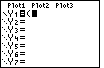
We start this sequence on the Y= screen by pressing
the  key. We start with the left parenthesis, key. We start with the left parenthesis,
 .
In order to insert the abs( we need to move first to the
TEST screen, via the .
In order to insert the abs( we need to move first to the
TEST screen, via the   key sequence. key sequence.
|
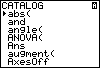
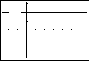
| Fortunately for us, the abs( item is the very first in the
CATALOG, as shown in Figure 2. The arrow pointer to the left of the abs( item
could be moved with the up and down cursor keys, but we do not
need to move it at all in this case. We press the  key to select this item and put it into the expression we were creting.
 |
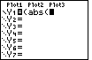
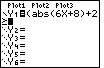
| Figure 3 shows the expression with the abs( pasted in from the CATALOG screen. |
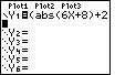
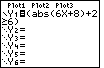
| In Figure 4 we have added more of the expression. We now need to enter the
symbol for "greater than or equal to". To do this we need to move to the
TEST menu via the  sequence. sequence. |
| Here is the test menu. The item we want is item number 4.
We need only press the  to select the item, close the
screen and insert the item into the expression. to select the item, close the
screen and insert the item into the expression. |
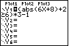
| Figure 6 confirms the insertion of the  symbol. symbol.
|
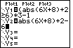
| We finish the expression in Figure 7. Each time this expression is evaluated it will produce a 0 if it is false, and a 1 if it is true. We wanted to change those values so that the graph does not fall on the X-axis. The opening and closing parentheses allow us to multiply the expression by 3 and then we can subtract 1. This will change false values to -1 and true values to 2. |
| Figure 8 shows the completed expression. We are ready to
graph the expression. To do this we press the  key. key. |
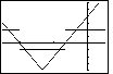
| Here is the graph of the solution.
We can see that the expression is true everywhere except from about -2 to about -2/3.
We can focus in on this region by changing the WINDOW settings.
To do this we press the  key. key.
|
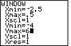
| Figure 10 shows the WINDOW settings after we have changed them to concentrate our graph on the region from -2.5 to 0.5. At the same time we have changed the Y-values to range from -4 to 6. |
| Pessing the key returns us to the
GRAPH screen shown in Figure 11. |
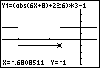
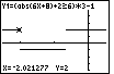
| For Figure 12 we have pressed the  key to move into the TRACE mode of the calculator, and we
have used the
key to move into the TRACE mode of the calculator, and we
have used the  key to move to the
right end of the lower segement of the graph. Note that the X-value
is -.6808511. If we had moved one more pixel to the right we would
jump up to the upper portion of the graph, and the X-value would be
greater than -2/3. If we wanted to, we could return to the WINDOW settings and change them
so that we examine just the region from -.68 to -.66, giving us an even
better reading of the X-values at the ends of the upper and lower
segments. For this example we will not do this. The graph here is meant to
confirm, to check, the algebraic solution in the text. key to move to the
right end of the lower segement of the graph. Note that the X-value
is -.6808511. If we had moved one more pixel to the right we would
jump up to the upper portion of the graph, and the X-value would be
greater than -2/3. If we wanted to, we could return to the WINDOW settings and change them
so that we examine just the region from -.68 to -.66, giving us an even
better reading of the X-values at the ends of the upper and lower
segments. For this example we will not do this. The graph here is meant to
confirm, to check, the algebraic solution in the text. |
| We can use the  key to
move the TRACE pointer to the left. In Figure 13 we have moved it until it has jumped to the
left upper portion of the graph. Again, we can see the X-value of the
particular pixel. key to
move the TRACE pointer to the left. In Figure 13 we have moved it until it has jumped to the
left upper portion of the graph. Again, we can see the X-value of the
particular pixel. |
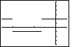
The final three figures on this page are meant to demonstrate the relation between what we say we are doing, and what we are really doing. The original problem was to solve
| In Figure 14 we have returned to the Y= screen and we have entered the new, unsimplified, equation. |
| We return to the GRAPH screen and we can see not only the original two level
function, but also the graph of our new function
|
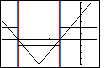
| The change from Figure 15 to Figure 16 is that we have drawn two red and
two blue vertical lines.
The red lines are above and below the endpoints of the lower level segment of the two level
function. That is, they mark the left and right ends of the region where the original
expression was false. The blue lines are above and below the endpoints of
the upper level segments of the two level function.
That is, they mark the right and left ends of the region where the original
expression was true. These red and blue lines were added to make it easier to see where the "V" graph of the second function is above the X-axis and where it is below the X-axis. |
©Roger M. Palay
Saline, MI 48176
February, 1999